Heat conduction with phase change (ice slab melting)

• Parabolic/T/1D_Two-phase_Stefan_problem_for_ice_melting/Two-phase_Stefan_problem.prj

Problem description

This benchmark is testing the extended version of a classical heat conduction equation termed ‘heat conduction equation with phase change’ (with a slight abuse of notations, we also call it simply ‘T+freezing’ equation). The initial-boundary value problem (IBVP) for this equation models such processes as ice formation and ice melting in water-saturated porous medium. Since the equation is strongly non-linear in the temperature variable $T$ to be solved for and contains multiple parameters which may affect accuracy of finite element discretization, a carefully designed model and code verification must be performed.

In this note, we consider the so-called two-phase Stefan problem which describes melting of a semi-infinite solid slab (in our case, an ice slab), and for which the closed-from analytical solution in $x\in(0,\infty)$ is available. We apply the IBVP for our T+freezing equation – with the porosity $\phi$ being set to 1 – to model such melting process and solve the problem in OpenGeoSys (OGS-6). This is done in a relatively large but finite spatial interval by extracting the initial condition, as well as the Dirichlet boundary conditions from the reference analytical data. The results obtained in this interval at various time-steps for the two modeling approaches are compared.

Test case in figures

The detailed Stefan problem description, geometric setup, material and model parameters used in the related OGS implementation can be found in this document this PDF. The figures below are taken from this documentation and serve for illustrative purposes to give a hint about the modeled process and simulations outcome.

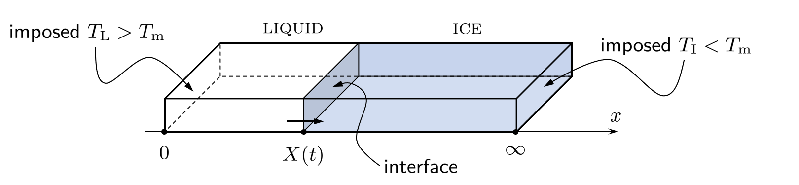
1. The sketch of a semi-infinite melting ice slab as a physical situation modeled be the two-phase Stefan problem:

   

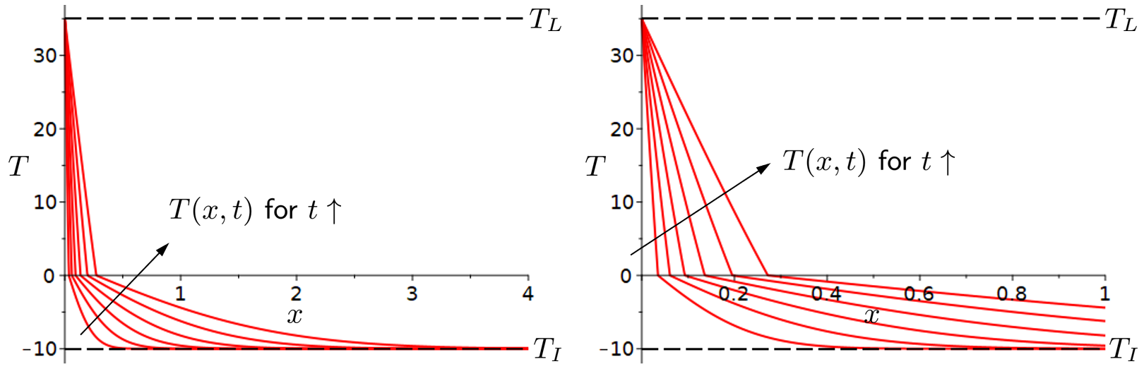
2. Plots of the analytical solution of Stefan problem restricted to finite spatial interval at fixed time steps (the left figure):

   

   This describes temperature evolution during the ice melting process within water and ice phases. The right figure zooms in at the solution in a smaller (in this case, unit) interval, which is to be used for comparison purposes. Temperature is given in degrees Celsius.
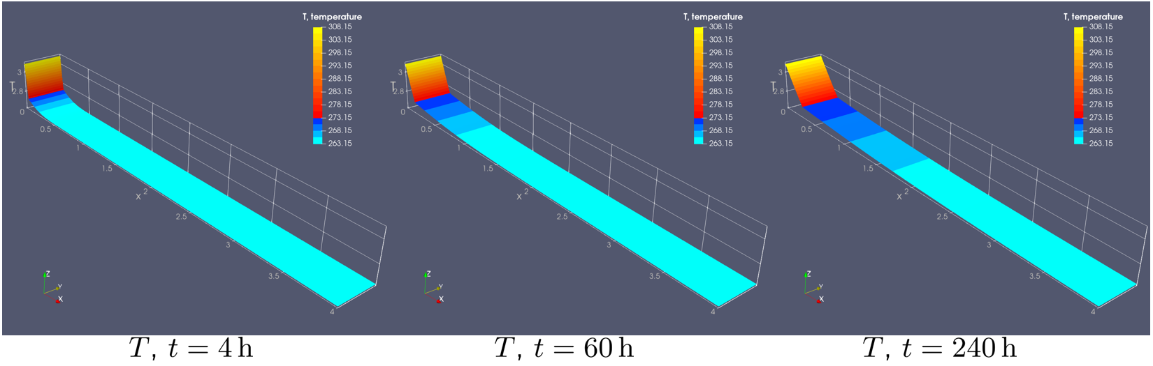
3. Sketches the OGS solution (a 3d view) of the IBVP for the ‘T+freezing’ equation at different time steps:

   

   Note that in these ParaView plots, we have tuned the color legend for temperature (here, given in kelvins) such that water and ice fractions can be identified more easily.
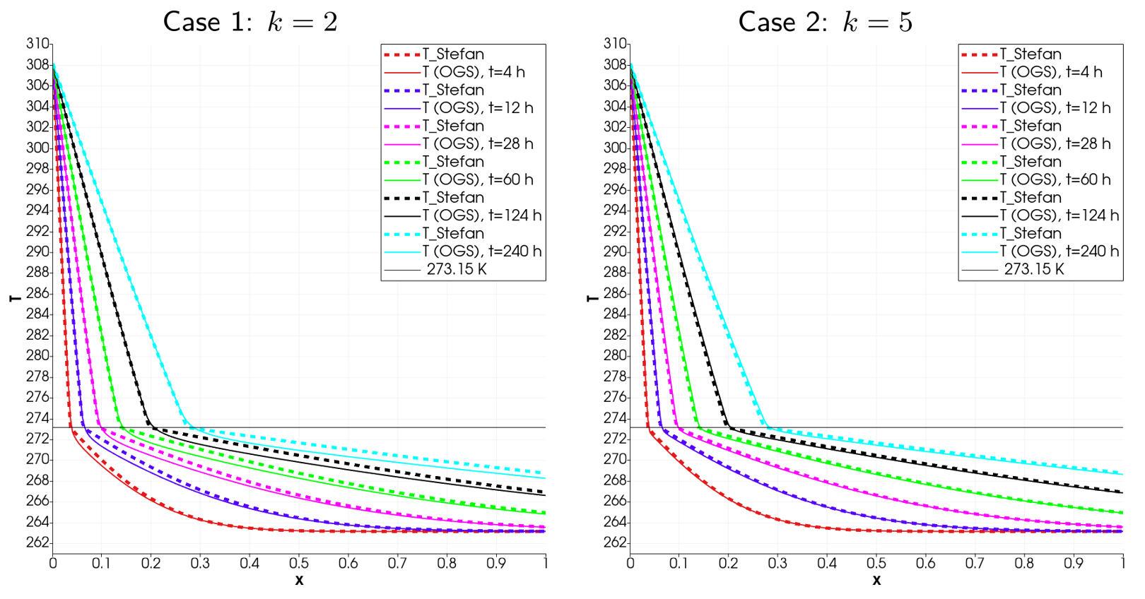
4. Finally, the figure below presents comparison of the analytical solution of Stefan problem and the OGS solution of the IBVP for the T+freezing equation obtained in two cases of a model parameter $k$ (it controls the thickness of a transition zone in a regularized ice-fraction indicator function and has impact on the discretization accuracy):

   

   In these plots, the temperature is given in kelvins as well.

Remark

In the corresponding OGS project file Two-phase_Stefan_problem.prj the time discretization is different for the “real case study” whose results are presented in the documentation and for the ctest case, and must be altered manually.