Heat conduction with phase change (soil freezing around BHE)

• Parabolic/T/2D_Soil_freezing_round_BHE/m16m15projectB.prj

Problem description

This benchmark is testing the extended version of a classical heat conduction equation termed ‘heat conduction equation with phase change’ (with a slight abuse of notations, we also call it simply ‘T+freezing’ equation). The initial-boundary value problem (IBVP) for this equation models such processes as ice formation and ice melting in water-saturated porous medium. Since the equation is strongly non-linear in the temperature variable $T$ to be solved for and contains multiple parameters which may affect accuracy of finite element discretization, a carefully designed model and code verification must be performed.

Below, we model heat transfer process – focusing specifically on ice formation – in a cylindrical soil specimen around a borehole heat exchanger (BHE) which contains a refrigerant of sub-zero temperature. This (negative) temperature is used to prescribe a Dirichlet boundary condition on the specimen boundary adjacent to the BHE, what triggers cooling and consequent freezing of water-saturated soil whose initial temperature is positive.

Simulations are performed using both our OpenGeoSys platform and the FreeFem++ open source finite element code (in the following, simply termed OGS and FF++, respectively), thus enabling cross-verification of the numerical codes.

Test case in figures

The detailed IBVP problem description for the T+freezing equation, geometric setup, material and model parameters used in the implementation can be found in this document this PDF document. The figures below are taken from this documentation and serve for illustrative purposes to give a hint about the modeled process and simulations outcome.

1. We assume the problem to be 3d-axisymmetric and hence opt for reducing it to 2-dimensional setting, as depicted in the figure below. A quarter of a cylindrical soil specimen around a BHE (a quarter of a 3-dimensional domain $\Omega$) and reduction to 2d computational domain $S$:

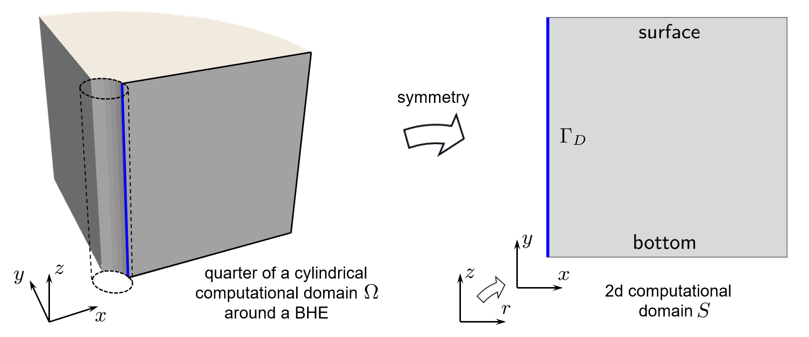
Note that $(r,z)\in S$ are denoted as $(x,y)$ which are assumed to be unrelated to the coordinate notations in the original 3d formulation. 2. The initial condition for $T$ in $S$ is assumed to be a positive function which decays linearly from surface to bottom. For modeling the (time-dependent) boundary conditions on $\Gamma_D$ of $S$, it is assumed that within the first $\widehat{t}$ hours, the temperature on $\Gamma_D$ drops continuously from the initial state to the values prescribed by some continuous piecewise linear function of $y$ and such that at the last depth segment it becomes negative. (The latter mimics the impact of the BHE refrigerant with sub-zero temperature.) The figure sketches the situation:

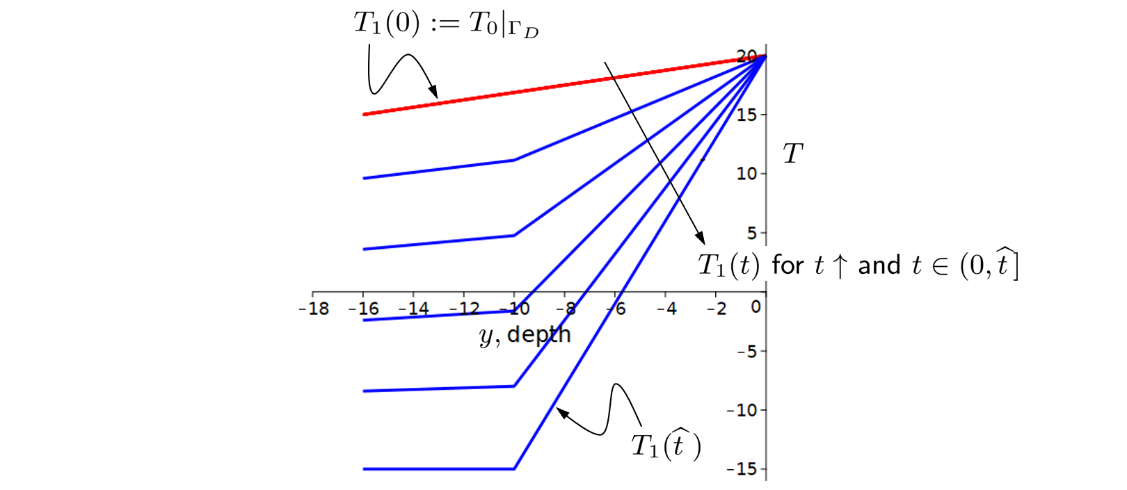
Temperature is given in degrees Celsius. For $t>\widehat{t}$, the prescribed temperature on $\Gamma_D$ and, thus, the heat conduction in the modelled case is triggered by a significant difference between the temperature on $\Gamma_D$ and the initial one within $S$. 3. The results of modelling are depicted in the following two figures, where we plot the temperature distribution in the soil block after 720 hours (30 days) of cooling, and also compare the outcomes of the two corresponding packages:

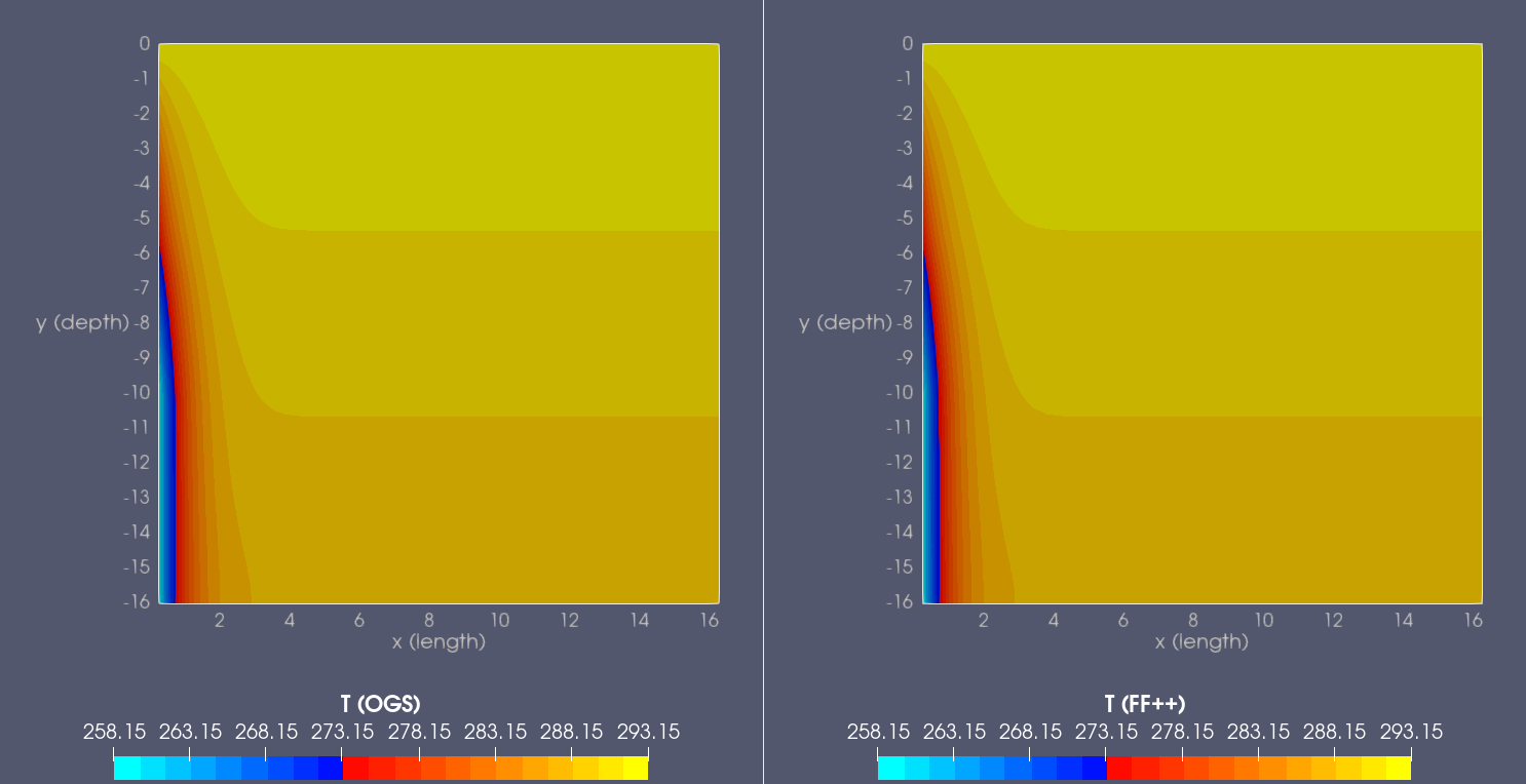
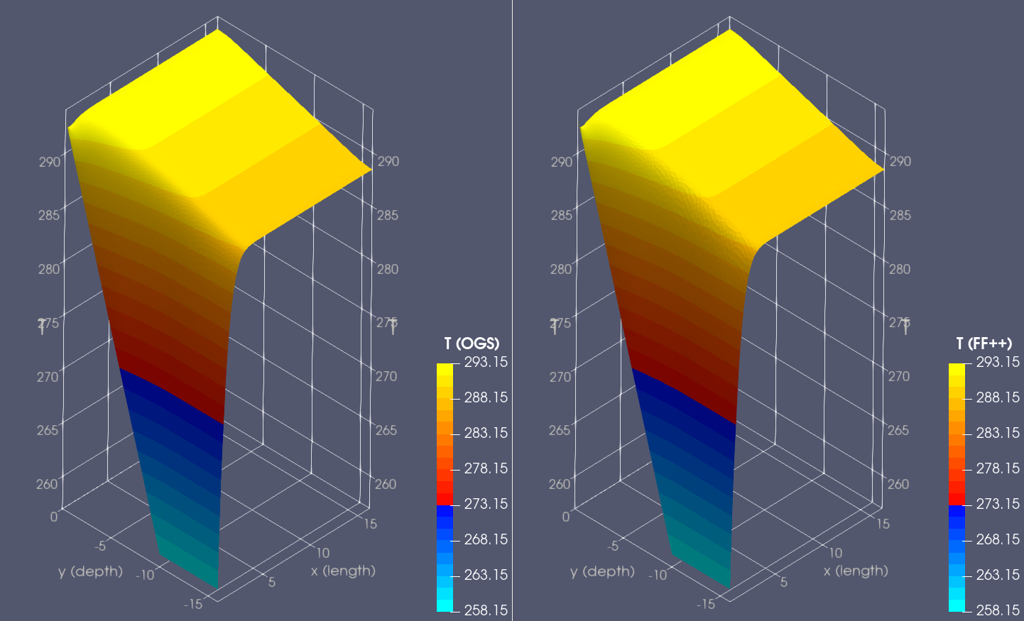
Temperature is given in kelvins. The color legend of $T$ in the corresponding ParaView plots is tuned such that the amount of ice formed around BHEs can be identified. As expected, ice formation occurs in the vicinity of $\Gamma_D$, more specifically, near the segment of $\Gamma_D$ in which the negative temperature has been prescribed. In the rest of the domain, temperature distribution remains almost identical to the initial state, as could also be expected. 4. Finally, the corresponding results from the previous figure are plotted over the three different directed lines within the domain $S$:

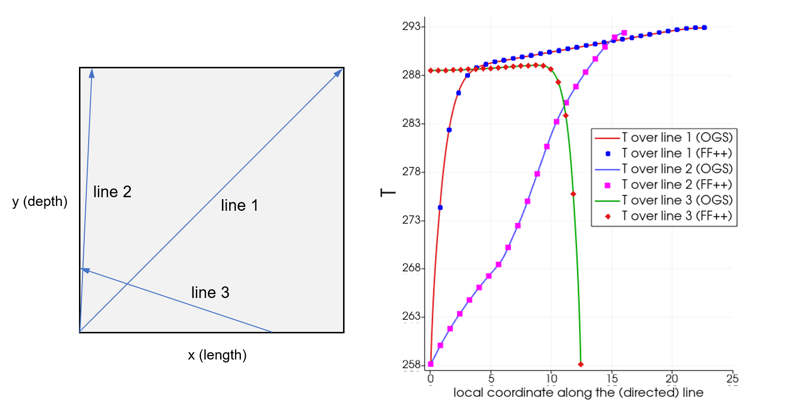
Here, origin of the horizontal axis on the right plot corresponds to line’s origin. For the selected lines, the compared data seems identical point-wise, thus supporting the quantitative similarity of the OGS and FF++ results observed earlier.

Remark

In the corresponding OGS project file m16m15projectB.prj the time discretization is different for the “real case study” whose results are presented in the documentation and for the ctest case, and must be altered manually.