BHE Array 2D
Problem description
When shallow geothermal energy is extracted by using Borehole Heat Exchanger (BHE) for heating of buildings, it causes the decrease of subsurface temperature in the vicinity of BHE. In this benchmark, a 2D numerical model has been constructed to model the above temperature variation. The model is validated against the super-imposed analytical solution. Additionally the impact of mesh density to the accuracy of numerical result is also discussed.
Analytical Solution
For the temperature change in an infinite homogeneous subsurface caused by one single BHE, it can be calculated by the line-source analytical solution (cf. Stauffer et al. (2013) , section 3.1.3), with the assumption that thermal conduction is the only process and no groundwater flow is present. In this case, the ground temperature $T$ is subject to the following equation.
\begin{equation} T-T_0 = \frac{q_b}{4\pi \lambda}E_1 \frac{r^2}{4\alpha t} \end{equation}
where $q_b$ is the heat extraction rate on the BHE and $E_1$ denotes the exponential integral function. $T_0$ refers to the initial ground Temperature, and $r$ is the distance between the observation point and the BHE.
In case multiple BHEs are present, Bayer et al. (2014) proposed to calculate the temperature change by super-impose the line-source model of equation (1). The overall temperature change at an observation point with a local coordinate (i, j) can be then calculated as
\begin{equation} \Delta \mathop T\nolimits_{i,j} \left( {t,\mathop q\nolimits_{k = 1,…,n} } \right) = \sum\limits_{k = 1}^n {\Delta \mathop T\nolimits_{i,j,k} } \left( {t,\mathop q\nolimits_k } \right). \end{equation}
where ${\mathop q\nolimits_k }$ is a sequence of heat extraction pulses at t =1, … ,m time steps. In this benchmark, the time step size of heat extraction pulses is set to 120 days, reflecting a 4-month long heat period and the 8-month long recovery interval every year. Within one time step the heat extraction rate on each BHE remains constant. By combining equation (1) and equation (2), the super-imposed temperature change due to the thermal load ${\mathop q\nolimits_k }$ imposed on each BHE can be calculated as
\begin{equation}\begin{split} \Delta \mathop T\nolimits_{i,j} \left( {t,\mathop q\nolimits_{k,l = 1,…,m} } \right)= \sum\limits_{k = 1}^m {\frac{{\mathop q\nolimits_l - \mathop q\nolimits_{l - 1} }}{{4\pi L\lambda }}} E_1\left[ {\frac{{{{\left( {i - \mathop x\nolimits_k } \right)}^2} + {{\left( {j - \mathop y\nolimits_k } \right)}^2}}}{{4\alpha \left( {\mathop t\nolimits_m - \mathop t\nolimits_l } \right)}}} \right] \ = \sum\limits_{l = 1}^m {\sum\limits_{k = l}^n {\frac{{\mathop q\nolimits_{k,l} }}{{4\pi L\lambda }}} } \left( {E_1\left[ {\frac{{{{\left( {i - \mathop x\nolimits_k } \right)}^2} + {{\left( {j - \mathop y\nolimits_k } \right)}^2}}}{{4\alpha \left( {\mathop t\nolimits_m - \mathop t\nolimits_{l - 1} } \right)}}} \right] - E_1\left[ {\frac{{{{\left( {i - \mathop x\nolimits_k } \right)}^2} + {{\left( {j - \mathop y\nolimits_k } \right)}^2}}}{{4\alpha \left( {\mathop t\nolimits_m - \mathop t\nolimits_l } \right)}}} \right]} \right). \end{split}\end{equation}
where ${\mathop q\nolimits_{k,l} }$ is the heat extraction of the k-th BHE at time step l. The equation (3) will be used to calculate the analytical solution of the overall temperature change in this model for validating the numerical results. It is written in python code and can be found here.
Numerical model setup
A 2D numerical model was constructed and simulated with the Finite element code OpenGeoSys (OGS). The subsurface was represented by a $100 \times 100~m$ square-shaped domain, inside of which 25 BHEs were installed (cf. Figure 1). The distance between adjacent BHEs is kept at 5 m. The ground temperature variation caused by the operation of the BHE array was simulated over a three years’ period. In the model, a 4-month heating period is assumed every year from January to April, with a constant heat extraction rate of 35 W/m on each BHE. In the rest months, the BHE system is shut down and no heat extraction was imposed. The parameters applied in the numerical model can be found in the table below.
In this model, the quad element was adopted to compose the mesh. The initial temperature of the model domain is set to 10 $^{\circ}$C. For the need of modelling a fixed 10 $^{\circ}$C temperature boundary condition was imposed at coordinate (0 m, 0 m). In the model domain, the locations of the BHEs are identified as red dots as in Figure 1. On each of these points, a sink term was specified in the numerical model, with the specific heat extraction rate as listed in the following table.
| Parameter | Symbol | Value | Unit |
|---|---|---|---|
| Soil thermal conductivity | $\lambda$ | $2.0$ | $Wm^{-1}K^{-1}$ |
| Soil heat capacity | $\rho c$ | $2.925\times10^{6}$ | $J^{-3} mK^{-1}$ |
| Ground thermal diffusivity | $\alpha$ | $5.7\times10^{-7}$ | $Wm^{-1}K^{-1}$ |
| Initial subsurface temperature | $T_0$ | $10$ | $^{\circ}C$ |
| Heat extraction rate of the BHE | $q$ | $35$ | $W/m$ |
| Diameter of the BHE | $D$ | $0.15$ | $m$ |
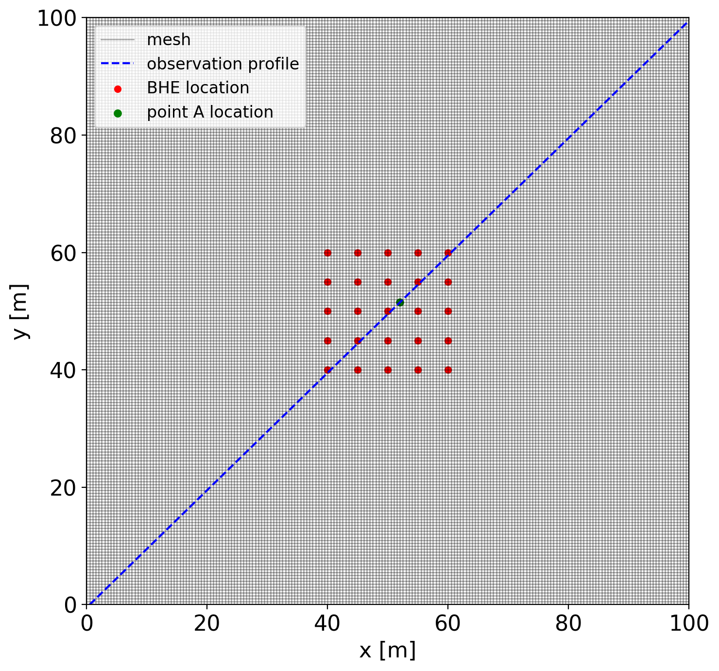
Model geometry, BHE location, and the observation profile
Different meshes were adopted to analyse the impact of mesh density on the numerical results. According to Diersch et al. (2011) the different element size can affect the accuracy of the numerical result significantly for such type of BHE simulation. The optimal element size $\triangle$ in a 2D model around the BHE node should have the following relationship with respect to the BHE diameter:
\begin{equation} \begin{split} \Delta = {\rm{ }}a{r_b},\ \hspace{6mm} \end{split} \end{equation} with \begin{equation*} a = 4.81 \hspace{2mm} for\hspace{2mm} n=4, \end{equation*} \begin{equation*} a = 6.13 \hspace{2mm} for\hspace{2mm} n=6, \end{equation*} \begin{equation*} a = 6.16 \hspace{2mm} for\hspace{2mm} n=8. \end{equation*}
where $r_b$ is the BHE radius. n denotes the number of surrounding nodes. n = 8 is typical for a squared grid meshes. In this study, the BHE diameter is assumed to be 0.15 m. Based on equation (4) the optimal element size should be set to approximately 0.5 m.
Numerical modelling results
Figure 2 and 3 show the comparison of the temperature distribution along the observation profile (position see Figure 1) using analytical solution with the numerical results from OGS-5 and OGS-6 for every 4 months in the whole simulated time. It shows the numerical solution has a very good agreement with the analytical solution.
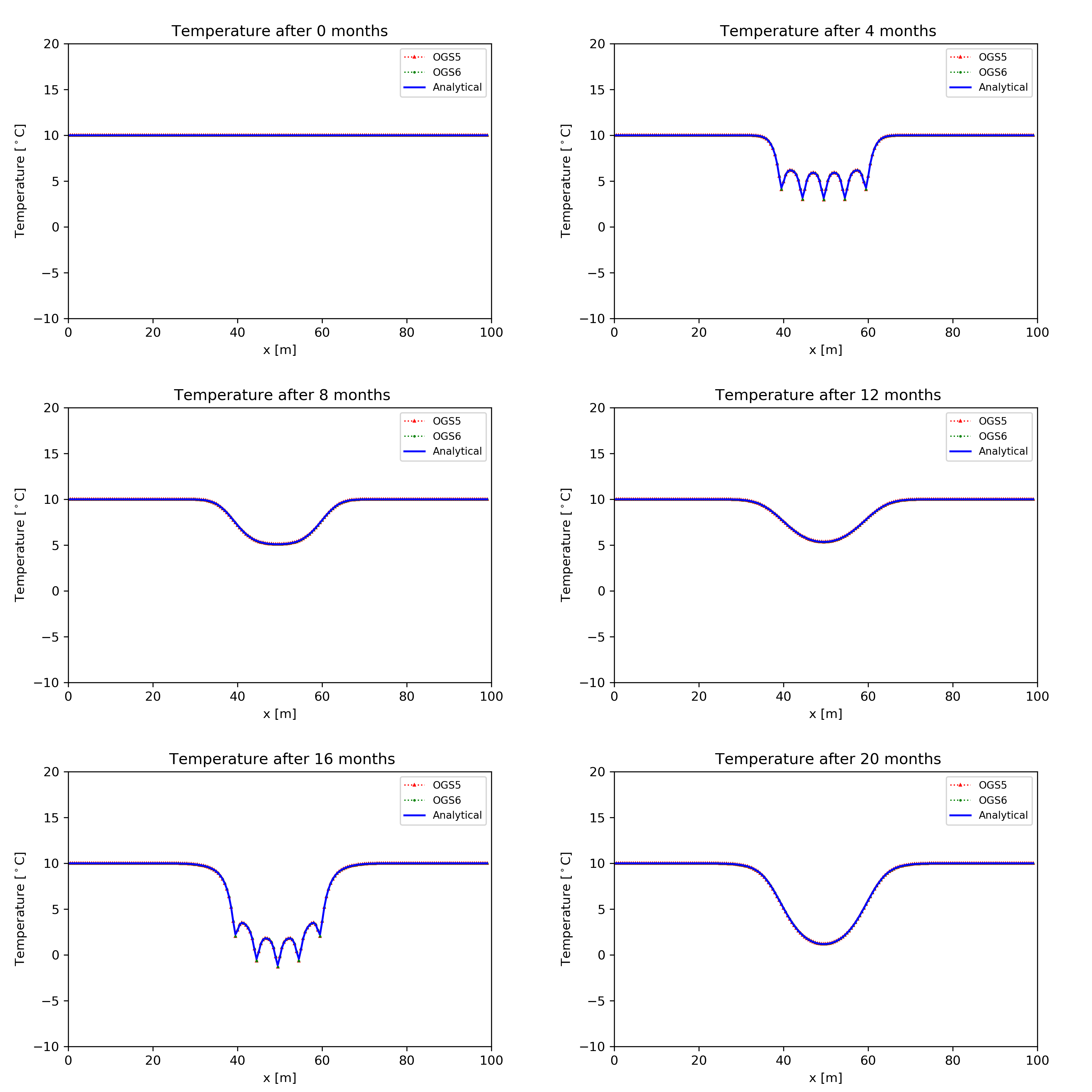
The temperature evolution of the BHEs field along the observation profile
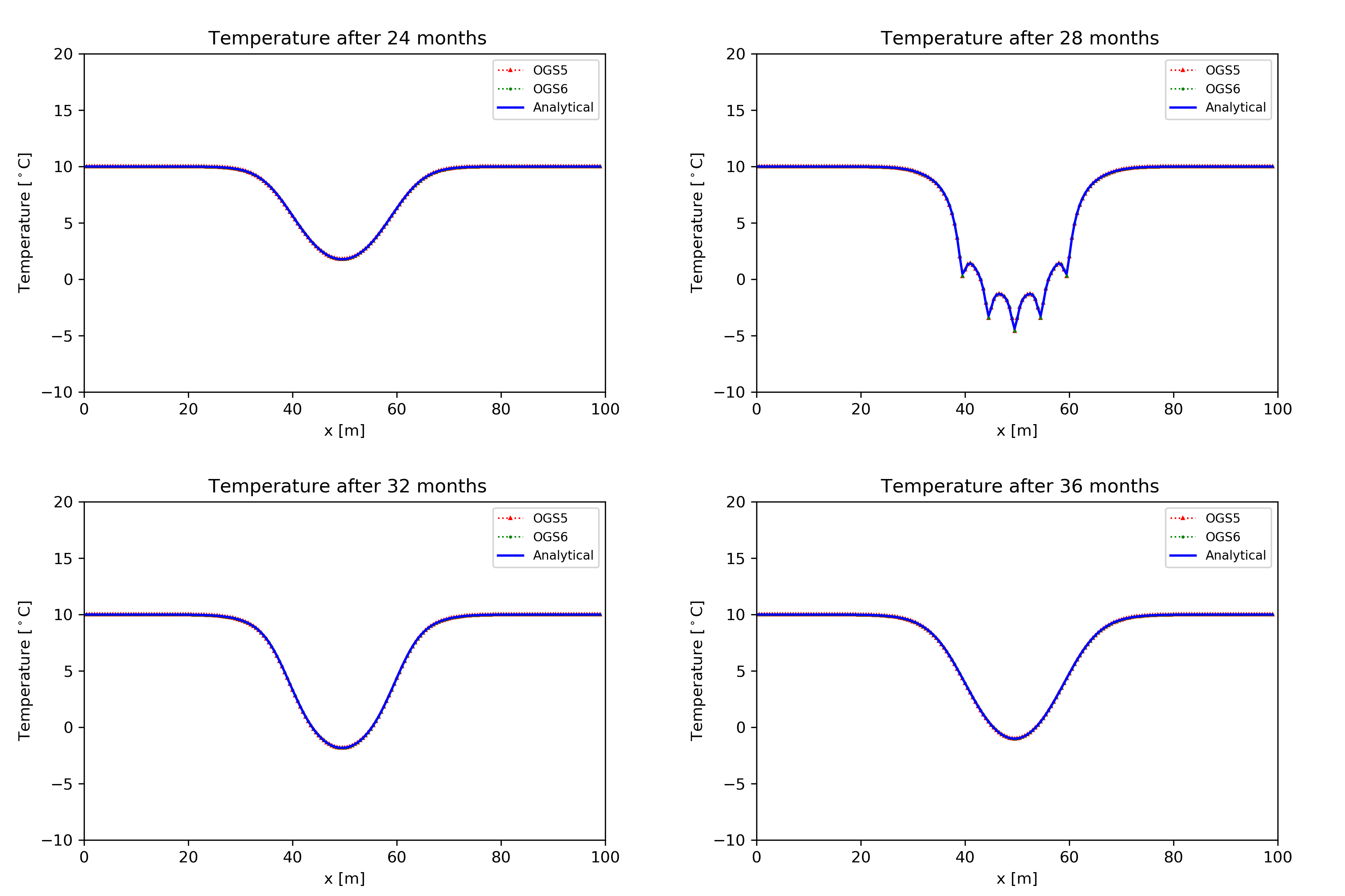
The temperature evolution of the BHEs field along the observation profile
In order to investigate the impact of mesh density on the accuracy of numerical result, the simulated temperature profile at the observation point A (53 m, 52.5 m) was plotted and compared against the analytical solution. Figure 3 shows the relative difference of the computed temperature between the analytical and numerical solution by using different mesh size (2.5 m, 1 m, 0.5 m, 0.25 m and 0.2 m). The results show that the difference becomes smaller when the mesh size is approaching 0.5 m, which is expected as the optimal mesh size mentioned in Diersch et al. (2011). From Figure 4, it can be found that the absolute error of temperature values at point A should be less than 2.5e-3 if the mesh size is kept denser than 0.5m.
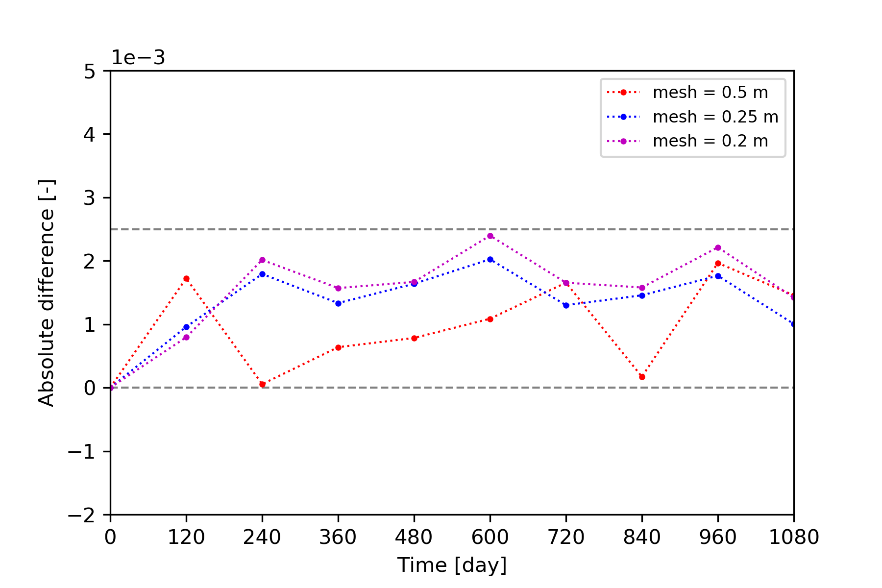
The relative difference of computed temperature at point A between the analytical and numerical solution using different mesh size
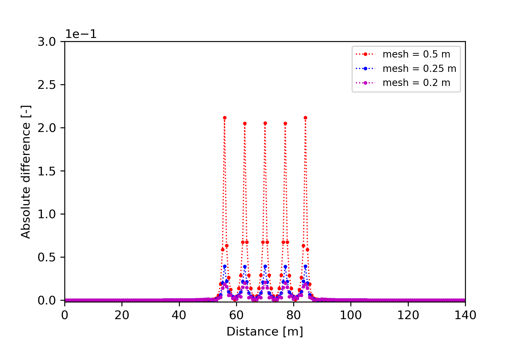
The absolute difference of computed temperature along the diagonal profile between the analytical and numerical solution using different mesh size
Summary
In this benchmark, a 2D numerical model has been constructed to simulate the ground temperature variation caused by heat extraction by BHE. The results show a very good agreement against the analytical solution. Additionally the impact of mesh density on the accuracy of numerical result was also investigated, and the optimal mesh size was found to be 0.5 m. In future studies, the pipe-line network system will be implemented into the model and coupled with the BHE.
References
[1] Bayer, P., de Paly, M., Beck, M., 2014. Strategic optimization of borehole heat exchanger field for seasonal geothermal heating and cooling. Applied Energy 136, 445-453. URL http://dx.doi.org/10.1016/j.apenergy.2014.09.029
[2] Diersch, H.-J., Bauer, D., Heidemann, W., Ruehaak, W., Schätzl, P., 2011. Finite element modeling of borehole heat exchanger systems: Part 2. Numerical simulation. Computers & Geosciences 37, 1136-1147.
[3] Stauffer, F., Bayer, P., Blum, P., Giraldo, N., Kinzelbach, W., 2013. Thermal Use of Shallow Groundwater. CRC Press, 290.
This article was written by Shuang Chen and Haibing Shao. If you are missing something or you find an error please let us know.
Generated with Hugo 0.122.0
in CI job 570044
|
Last revision: April 17, 2025
Commit: Rewrite using ranges 1ed34f4
| Edit this page on