Heatconduction (Neumann)
Equations
We consider homogeneous parabolic equation here:
$$ \begin{equation} \rho C_\textrm{p}\frac{\partial T}{\partial t} + \nabla\cdot(\lambda \nabla T) = 0 \quad \text{in }\Omega \end{equation}$$w.r.t boundary conditions
$$ \eqalign{ T(x, t=0) = T_0,\cr T(x) = g_D(x) &\quad \text{on }\Gamma_D,\cr \lambda {\partial T(x) \over \partial n} = g_N(x) &\quad \text{on }\Gamma_N, } $$where $T$ could be temperature, the subscripts $D$ and $N$ denote the Dirichlet- and Neumann-type boundary conditions, $n$ is the normal vector pointing outside of $\Omega$, and $\Gamma = \Gamma_D \cup \Gamma_N$ and $\Gamma_D \cap \Gamma_N = \emptyset$.
Problem specification and analytical solution
We solve the parabolic equation on a line domain $[60\times 1]$ with $\lambda = 3.2$ and $\rho C_\textrm{p} = 2.5 \times 10^6$ w.r.t. the specific boundary conditions:
$$ \eqalign{ \lambda {\partial T(x) \over \partial n} = q &\quad \text{on } (x=0) \subset \Gamma_N.\cr \lambda {\partial T(x) \over \partial n} = 0 &\quad \text{on } (x=60) \subset \Gamma_N. } $$with flux value being $q = 2$.
Approximate solution of this problem is the solution for semi-infinite rod, which is applicable as long as the temperature does not come close to the right side of the domain:
$$ \begin{equation} T(x,t) = \frac{2q}{\lambda}\left(\left(\frac{\alpha t}{\pi}\right)^{\frac{1}{2}} e^{-x^2/4\alpha t} - \frac{x}{2}\textrm{erfc}\left( \frac{x}{2\sqrt{\alpha t}}\right)\right), \end{equation} $$where $T_\textrm{b}$ is the boundary temperature, $\textrm{erfc}$ is the complementary error function and $\alpha = \lambda/(C_p \rho)$ is the thermal diffusivity.
Input files
The main project file is picard.prj. It describes the processes to be solved and the related process variables together with their initial and boundary conditions. It also references the mesh and geometrical objects defined on the mesh.
The geometries used to specify the boundary conditions are given in the
line_60_geometry.gml file. The input mesh is stored in the mesh.vtu file.
Same project was also setup to be solved with the Newton-Raphson method, see
newton.prj input file.
Another two project files were tested with a mass-lumping method used to
reduce oscillations for particularly small ratios of element size to time step
increment. See picard_masslumping.prj and newton_masslumping.prj files.
Results and evaluation
Picard vs. Newton
For the simple equation, as expected, the difference between the Picard and Newton non-linear solvers is reasonable for the given non-linear solver tolerances.
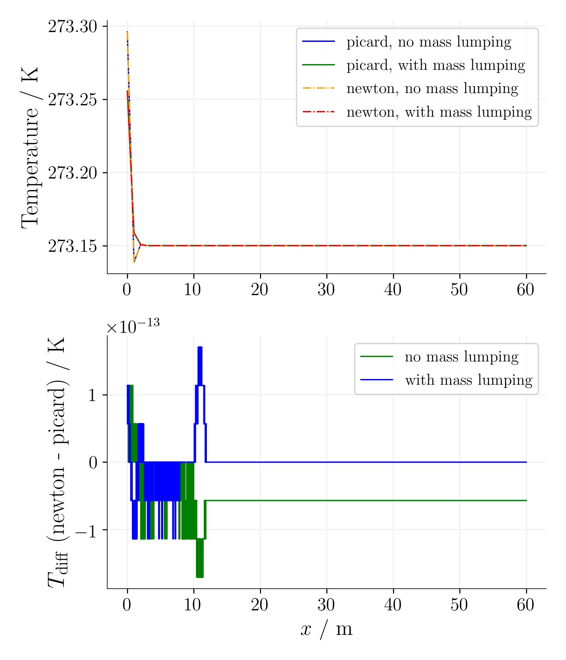 Time step 1, time 78125s. |
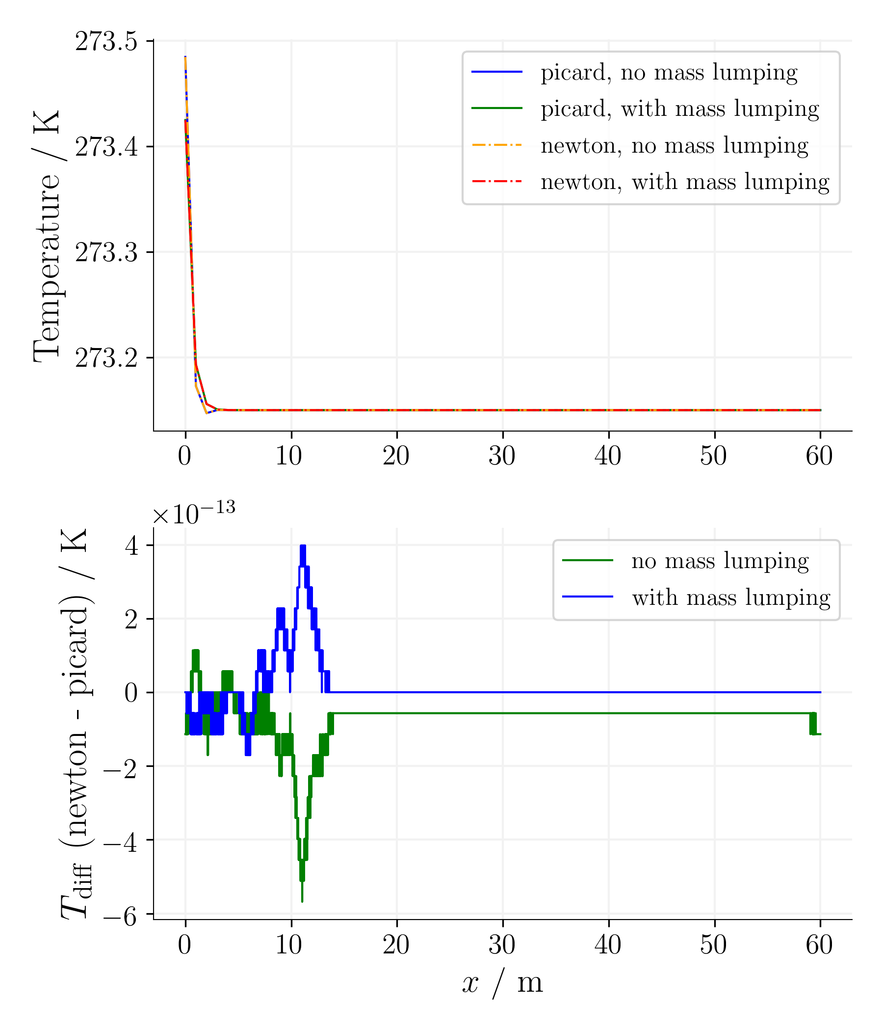 Time step 3, time 234375s. |
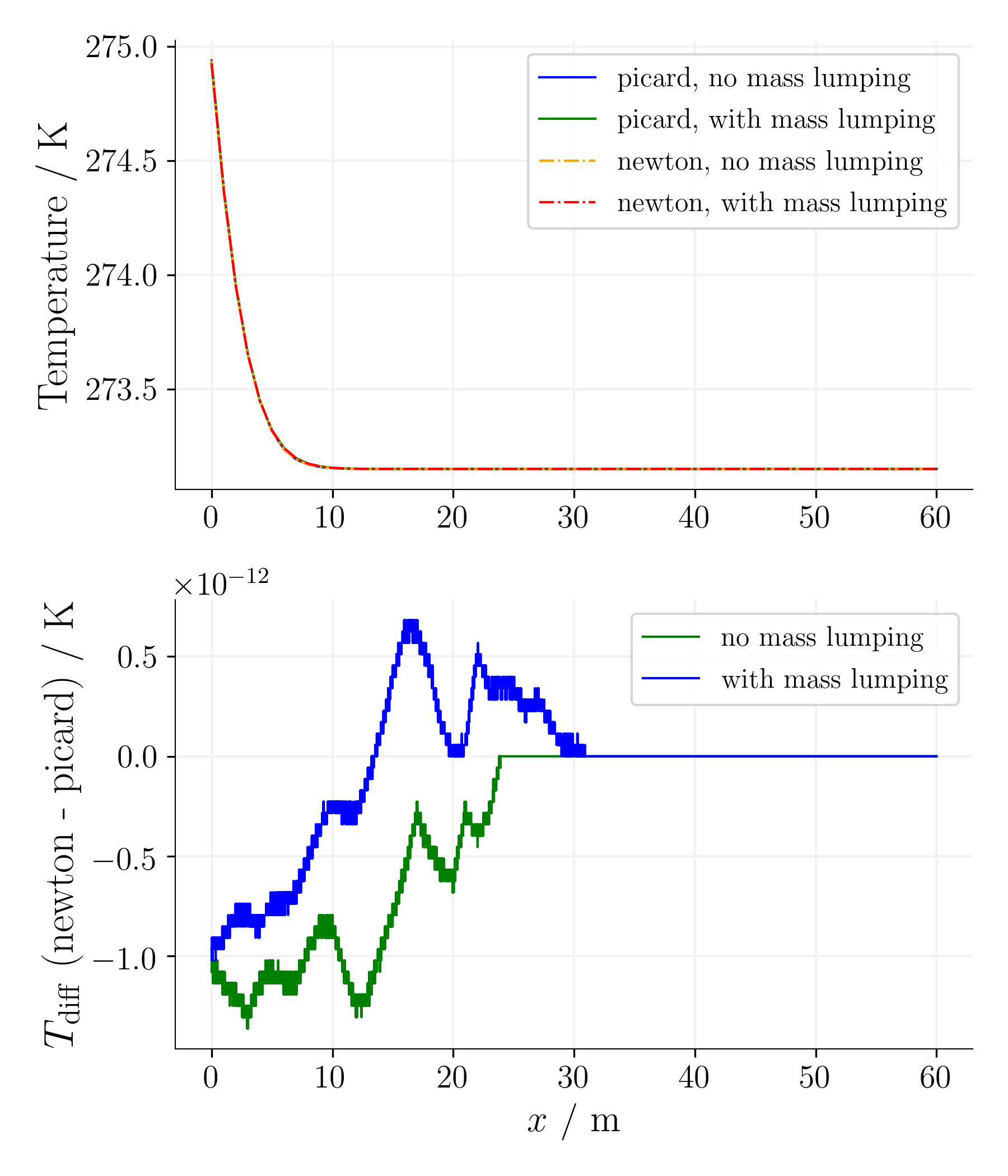 Time step 65, time 5078125s. |
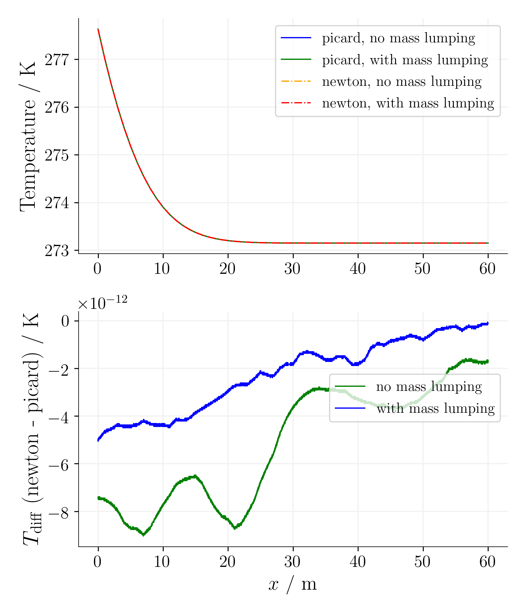 Time step 405, time 31640625s. |
Mass-lumping and analytical solution
Using the mass-lumping method reduces the oscillations for the first time steps on cost of accuracy as the error is significantly larger.
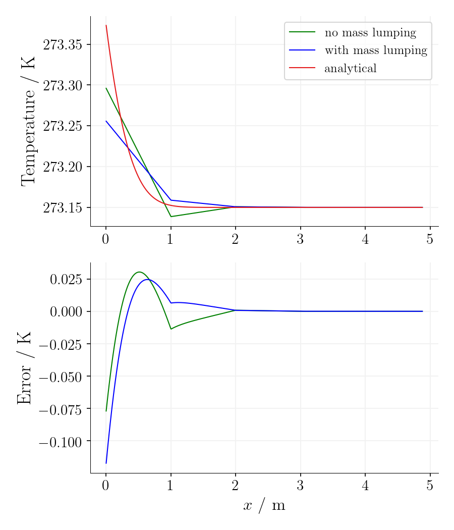 Time step 1, time 78125s. |
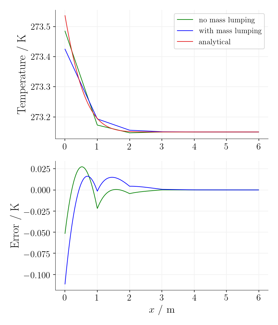 Time step 3, time 234375s. |
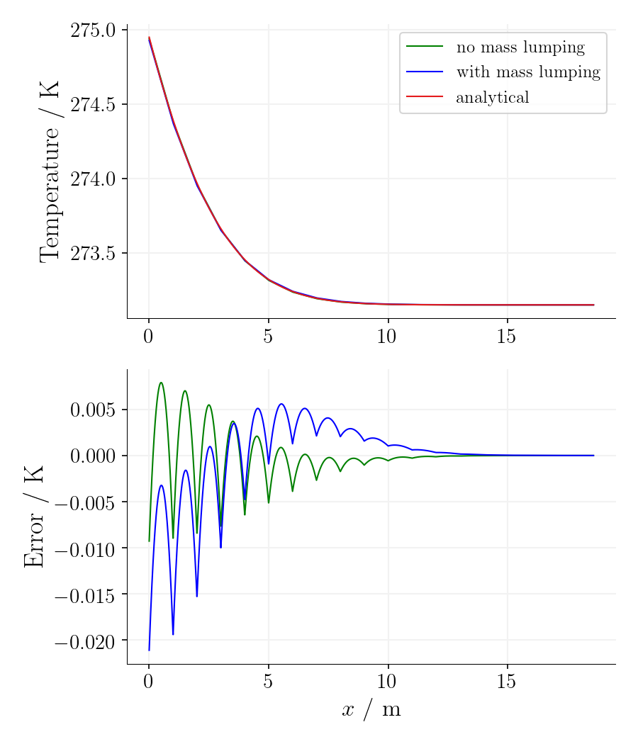 Time step 65, time 5078125s. |
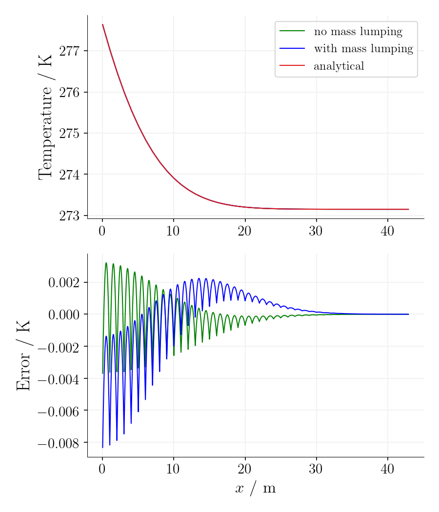 Time step 405, time 31640625s. |
This article was written by Dmitri Naumov, Tianyuan Zheng. If you are missing something or you find an error please let us know.
Generated with Hugo 0.147.9
in CI job 683680
|
Last revision: December 20, 2025
Commit: chore: fix spelling mistakes fbc5f730
| Edit this page on