HEAT_TRANSPORT_BHE

Description

Borehole heat exchangers (BHE) are widely applied in Ground Source Heat Pump (GSHP) systems to explore geothermal energy for building heating and cooling purposes. There are more and more engineering companies starting to use simulation tools for the performance evaluation and design of GSHP projects.
For OGS-6, it allows the users to simulate the subsurface and soil temperature evolution induced by BHE and operation performance of BHE coupled heat pump.

Mathematical framework

This part aims to give an explanation of the mathematical framework in configuring the HEAT_TRANSPORT_BHE process provided in OpenGeoSys. The numerical method implemented in OGS-6 is the so-called double-continuum finite element method (DC-FEM). This approach was originally proposed by Al-Khoury et al. (2010) and extended by Diersch et al. (2011a; 2011b). It was then implemented in OpenGeoSys by Shao et al. (2016). This modelling approach has the following assumptions.

• The subsurface is considered to be a 3D continuum, while the BHE is represented by 1D line elements as the second continuum.
• The heat transfer between different BHE components is simulated by the Capacity-Resistance-Model (CaRM) in analogy to the electrical circuits.
• In the subsurface continuum, both heat convection and heat conduction are governed by the thermal energy conservation equation, and it reads:

Here, $\Lambda_s$ denotes the tensor of thermal hydrodynamic dispersion and $H_s$ represents the heat source and sink term.

• In the borehole continuum, each pipe is assigned with one governing equation, with the thermal convection in the pipeline simulated. Also, for each grout zone surrounding the pipeline, the thermal conduction equation was simulated. For details of the coupling between different borehole components and continua, interested readers may refer to Diersch et al. (2011a; 2011b).

Input parameters

In the configuration of HEAT_TRANSPORT_BHE process, it is generally configured as follows.

• <name>: should be HeatTransportBHE.
• <type>: should be HEAT_TRANSPORT_BHE.
• <integration_order>: It is the order of the integration method for element-wise integration, normally set to 2.
• <process_variables>: The primary variables of the HEAT_TRANSPORT_BHE process are temperature_soil and temperature_BHE1. For multiple boreholes, the name temperature_BHE2, temperature_BHE3 etc can be added.

<name>HeatTransportBHE</name>
<type>HEAT_TRANSPORT_BHE</type>
<integration_order>2</integration_order>
<process_variables>
    <process_variable>temperature_soil</process_variable>
    <process_variable>temperature_BHE1</process_variable>
</process_variables>

<borehole>

The borehole <length> and <diameter> are defined here. The unit of these parameters are in $\mathrm{m}$. Here is an example of a borehole with 18 m in length and 0.13 m in diameter.

<borehole>
    <length>18.0</length>
    <diameter>0.13</diameter>
</borehole>

<type>

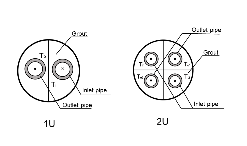
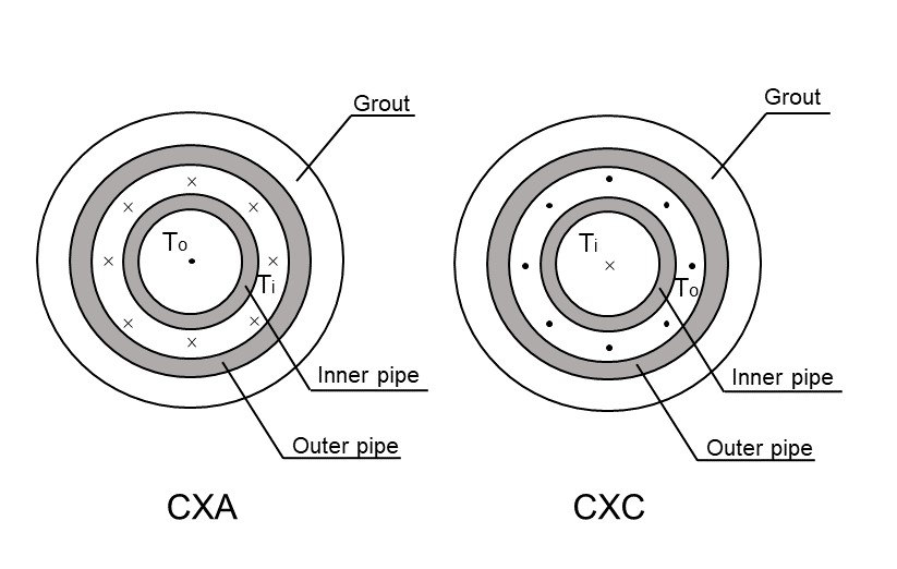
Currently there are 4 types of BHE available. Following the convention in Diersch et al. (2011a), they are named as 1U，2U，CXA and CXC types. In the OGS .prj file, it is defined as:

<type>2U</type>

• 1U: means there is only one single U-tube installed in the borehole;
• 2U: double U-tubes installed in the borehole;
• CXA: coaxial pipe with annular space as the inlet downwards flow and the centre part as outlet upwards flow;
• CXC: coaxial pipe with a reversed flow direction to CXA type.

Especially in CXA and CXC type, the direction of the borehole itself could be deviated by any angle, which is defined by mesh. The inflow direction will be in accordance with the direction of the line element (represents the BHE borehole) in the mesh. And the outlet direction is the opposite of the inflow direction.

The cross-sections of these 4 types of BHEs are illustrated in the following figures.

<pipes>

The properties of the pipes are defined in this section. For different types of BHE, the pipes are also configured differently.

• For coaxial pipes (CXA or CXC), <longitudinal_dispersion_length> should be given.
• For 1U and 2U type pipe, the <distance_between_pipes> must be given, along side with the <longitudinal_dispersion_length>.

The units of these parameters are all in $\mathrm{m}$. Here is an example of a 2U type BHE. The inlet and outlet pipe are all made of high-density polyethylene (HDPE).

<pipes>
    <inlet>
        <diameter> 0.0378</diameter>
        <wall_thickness>0.0029</wall_thickness>
        <wall_thermal_conductivity>0.42</wall_thermal_conductivity>
    </inlet>
    <outlet>
        <diameter>0.0378</diameter>
        <wall_thickness>0.0029</wall_thickness>
        <wall_thermal_conductivity>0.42</wall_thermal_conductivity>
    </outlet>
    <distance_between_pipes>0.053</distance_between_pipes>
    <longitudinal_dispersion_length>0.001</longitudinal_dispersion_length>
</pipes>

<flow_and_temperature_control>

Four type of flow and temperature control patterns are provided in OGS.

• FixedPowerConstantFlow:
  It means the BHE has a fixed thermal load and the refrigerant flow rate in the borehole is kept as a constant. The fixed heating load value was defined by the key word <power> , and the flow rate is given by <flow_rate>.
• FixedPowerFlowCurve:
  It means the BHE has a fixed thermal load and the flow rate is following a time dependent curve. The key word <power> is kept the same, while the flow rate is defined by a curve in the <curves>.
• PowerCurveConstantFlow:
  It means BHE has a constant flow rate while the power is various following a curve. The key word <flow_rate> applies here, along with the curve defined in the <curves>.
• TemperatureCurveConstantFlow:
  It means BHE has a constant <flow_rate> while the inflow temperature following the values defined in the <curves>.
• TemperatureCurveFlowCurve:
  It means both the BHE inflow rate and temperature values are following the corresponding curves.
• PowerCurveFlowCurve:
  It means both the BHE thermal load and flow rate values are following the corresponding curves.
• BuildingPowerCurveConstantFlow:
  It means the BHE thermal load is following a building heat load depending on a COP curve while the flow rate is kept as a constant.

The unit of <power> is in $\mathrm{W}$ and <flow_rate> is in $\mathrm{m^{3}/s}$. For heating applications, thermal energy is extracted from the subsurface, then a negative power value should be given. It is vice versa for cooling applications.

Further info:

For all the flow and temperature control options, OpenGeoSys calculates the inlet temperature of each BHE internally. For each BHE, temperature on its inlet pipe is always set as a Dirichlet type boundary condition. Depending on the choice of <flow_and_temperature_control>, the inflow temperature will be calculated dynamically in each time step and iteration to satisfy the given constrains.

Here is an example using TemperatureCurveConstantFlow.

<flow_and_temperature_control>
    <type>TemperatureCurveConstantFlow</type>
    <flow_rate>2.0e-4</flow_rate>
    <temperature_curve>inflow_temperature</temperature_curve>
</flow_and_temperature_control>

For 2U-type BHE configuration, the flow rate in <flow_and_temperature_control> indicates the flow rate within each U-pipe. When a fixed power or power curve is imposed on a 2U-type BHE, the given value in <flow_and_temperature_control> or in the related power curve should be specified with half of the user’s presumed entire borehole exchanger power.

<grout>

The thermal properties of the grout material is defined here.

• density: density of grout which has the unit of $\mathrm{kg/m^{3}}$;
• porosity: porosity of grout which is dimensionless;
• specific_heat_capacity: specific heat capacity of grout which has the unit of $\mathrm{J·kg^{-1} K^{-1}}$;
• thermal_conductivity: thermal conductivity of grout which has the unit of $\mathrm{W·m^{-1} K^{-1}}$.

Here is an example how the typical parameters of borehole grout looks like.

<grout>
    <density>2190.0</density>
    <porosity>0.0</porosity>
    <specific_heat_capacity>1735.1</specific_heat_capacity>
    <thermal_conductivity>0.73</thermal_conductivity>
</grout>

<refrigerant>

The thermal properties of the circulating fluid is defined here. The parameters and their units are listed below.

• density: density of circulating fluid, in the unit of $\mathrm{kg/m^{3}}$;
• viscosity: dynamic viscosity of circulating media which has the unit of $\mathrm{kg·m^{-1} s^{-1}}$;
• specific_heat_capacity: specific heat capacity of circulating fluid, which has the unit of $\mathrm{J·kg^{-1} K^{-1}}$;
• thermal_conductivity: thermal conductivity of the circulating fluid, which has the unit of $\mathrm{W·m^{-1} K^{-1}}$;
• reference_temperature: When the <flow_and_temperature_control> was not set to TemperatureCurveConstantFlow, OGS needs to have an initial outlet temperature value in the first time step to start the simulation. A reference temperature has to be defined for the calculation of initial inflow temperature. The unit of reference temperature is in $^{\circ}$C.

Here is an example in which the circulating fluid is water at about 15 $^{\circ}$C.

<refrigerant>
    <density>998</density>
    <viscosity>0.0011375 </viscosity>
    <specific_heat_capacity>4190</specific_heat_capacity>
    <thermal_conductivity>0.6</thermal_conductivity>
    <reference_temperature>22</reference_temperature>
</refrigerant>

Available Nonlinear Solvers

In the HEAT_TRANSPORT_BHE process, both Picard and Newton nonlinear solvers are supported. With the Picard solver, the linear equation system is iterated until the change in the solution vector is small enough (typically less than 1E-6). With the Newton approach, the global Jacobian matrix and residual vector are evaluated in each iteration, in order to solve for the change of solution vector in each iteration. The solved change vector is then further used to update the global solution vector. Typically, after 5 to 8 iterations, the Newton approach leads to a globally converged solution, i.e. the norm of the residual vector is less than certain tolerance (e.g. relative tolerance less than 1E-10). When configuring an OGS project with the HEAT_TRANSPORT_BHE process, Picard iterations will be sufficient when the time step size is kept small (tens of seconds). However, when the time step is large (hours or days), Newton iterations may reach convergence much faster than the Picard approach.

For more information regarding how to configure the Picard and Newton nonlinear solvers, please also refer to the section in Project File - Building Blocks

References

[1] Al-Khoury, R., Kölbel, T., Schramedei, R.: Efficient numerical modeling of borehole heat exchangers. Comput. Geosci. 36(10), 1301–1315 (2010).

[2] Diersch, H.-J.G., Bauer, D., Heidemann, W., Rühaak, W., Schätzl, P.: Finite element modeling of borehole heat exchanger systems: part 1. Fundamentals. Comput. Geosci. 37(8), 1122–1135 (2011a).

[3] Diersch, H.-J.G., Bauer, D., Heidemann, W., Rühaak, W., Schätzl, P.: Finite element modeling of borehole heat exchanger systems: part 2. Numerical simulation. Comput. Geosci. 37(8), 1136–1147 (2011b).

[4] Hein, P., Kolditz, O., Görke, U.-J., Bucher, A., Shao, H.: A numerical study on the sustainability and efficiency of borehole heat exchanger coupled ground source heat pump systems. Appl. Therm. Eng. 100, 421–433 (2016).

[5] Shao, Haibing, Philipp Hein, Agnes Sachse, and Olaf Kolditz. Geoenergy modeling II: shallow geothermal systems. Springer International Publishing, 2016.