LF process: Axisymmetric Theis solution (Pumping well)

import os
from pathlib import Path

import matplotlib.pyplot as plt
import numpy as np
import ogstools as ot
from scipy.special import exp1

Problem description

Theis problem examines the transient lowering of the water table induced by a pumping well. The assumptions required by the Theis solution are:

The aquifer:

• is homogeneous, isotropic, confined, and infinite in radial extent,
• has a uniform thickness and a horizontal piezometric surface.

The well:

• is fully penetrating the entire aquifer thickness,
• has a constant pumping rate,
• well storage effects can be neglected,
• no other wells or long-term changes in regional water levels.

Analytical solution

The analytical solution of the drawdown as a function of time and distance is expressed by:

where

• $s$ [$L$] is the drawdown or change in hydraulic head,
• $h_0$ is the constant initial hydraulic head,
• $h$ is the hydraulic head at distance $r$ at time $t$,
• $Q$ [$L^3T^{-1}$] is the constant pumping (discharge) rate,
• $S$ [$-$] is the depth-integrated aquifer storage coefficient (volume of water released per unit decrease in $h$ per unit area),
• $T$ [$L^2T^{-1}$] is the transmissivity (a measure of how much water is transported horizontally per unit time).

The Well Function, $W(u)$ is the exponential integral, $E_1(u).$ $W(u)$ is defined by an infinite series:

where $\gamma=0.577215664$ is the Euler-Mascheroni constant.

Simplification In this notebook we stick to the exact expression introduced above. However, in some practical applications, an approximation to the exponential integral is used:

This results in an expression for $s(r,t)$ known as the Jacob equation:

For more details we refer to Srivastava and Guzman-Guzman (1998).

def calc_u(r, S, T, t):
    """Calculate and return the dimensionless time parameter, u."""
    return r**2 * S / 4 / T / t


def theis_drawdown(t, S, T, Q, r):
    """Calculate and return the drawdown s(r,t) for parameters S, T.

    This version uses the Theis equation, s(r,t) = Q * W(u) / (4.pi.T),
    where W(u) is the well function for u = Sr^2 / (4Tt).
    S is the aquifer storage coefficient: S_0 * thickness,
    T is the transmissivity (m2/s): hydraulic conductivity * thickness,
    r is the distance from the well (m), and
    Q is the pumping rate (m3/s).
    """
    u = calc_u(r, S, T, t)
    return Q / 4 / np.pi / T * exp1(u)

Problem parameterisation

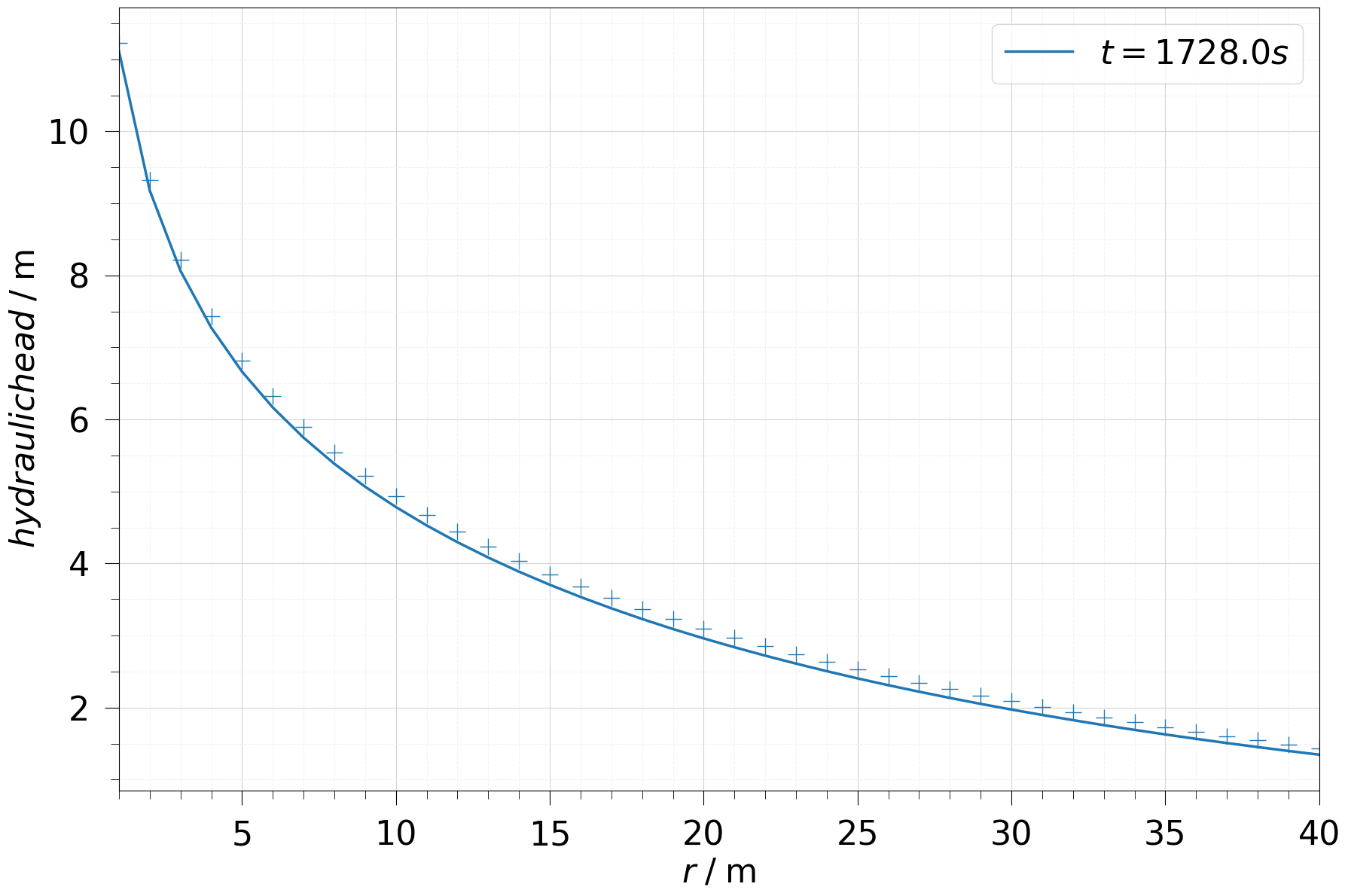
Here, we parameterise the problem to evaluate the Theis analytical solution against simulation results of OGS.

We set the pumping rate to $Q=0.016\,\mathrm{m^{3}/s}$ and consider the solution at time $t=1728.0\,\mathrm{s}$.

For the aquifer properties, we use a storativity of $S=1 \times 10^{-3}$ and a transmissivity of $T=1000\, \mathrm{m^{2}/day}$.

We show the drawdown over radial distances ranging from $r=1\,\mathrm{m}$ to $40\,\mathrm{m}$.

# Aquifer properties
#
# Storativity (-)
S = 0.001
# Transmissivity (m2/s)
T = 9.2903e-4

# Dynamic parameters
#
# Pumping rate from well (m3/s)
Q = 0.016

Evaluation

# Evaluation parameters
#
# Distance from well (m)
r = np.arange(1, 41, 1)
# Time values (s)
time_vals = [1728.0]

# Compute analytical solutions for the given time and distance values
len_time_vals = len(time_vals)
s_all = np.zeros((40, len(time_vals)))

for ii in range(len_time_vals):
    u = calc_u(r, S, T, time_vals[ii])
    s = theis_drawdown(time_vals[ii], S, T, Q, r)
    s_all[:, ii] = s

# Prepare output directory
out_dir = Path(os.environ.get("OGS_TESTRUNNER_OUT_DIR", "_out"))
out_dir.mkdir(parents=True, exist_ok=True)

sim = ot.Model(project="axisym_theis.prj").run(out_dir, overwrite=True)

# Load simulation results
ms = sim.meshseries

# Extract probe at y=z=0 and x=1..40
xaxis = np.column_stack((np.linspace(1.0, 40, 40), np.zeros((40, 2))))
pressure = ot.variables.pressure.replace(
    data_unit="m", output_unit="m", output_name="hydraulic head", symbol=""
)

ms_probe = ms.probe(xaxis)

# Plot results
labels = [f"$t={np.round(x, 2)}s$" for x in ms_probe[1:].timevalues]
fig, ax = plt.subplots(figsize=(18, 12))

ot.plot.line(ms_probe[1:], "x", pressure, labels=labels, ax=ax)
ax.plot(r, s_all, "+", markersize=16)
ax.set(
    xlim=(1, 40),
    xlabel=r"$r\;/\; \mathrm{m}$",
    ylabel=r"$hydraulic head \; /\; \mathrm{m}$",
)

fig.tight_layout()

# Validate results at time = 1728 s
time = 1728.0
timestep = ms_probe.closest_timestep(time)

analytical_solution = s_all[:, timestep - 1]

assert time == time_vals[timestep - 1]

abs_error = np.abs(analytical_solution - ms_probe.point_data[pressure][timestep])

rel_error = np.abs(abs_error / analytical_solution)

np.testing.assert_array_less(abs_error, 0.2)
np.testing.assert_array_less(rel_error, 0.07)

Solutions at later time steps computed by OGS6 deviate from the analytical solution because of two reasons:

• the time discretisation of the numerical model is chosen too coarse
• the solution of Theis assumes an aquifer of infinite radial extent wich for larger times deviates more visibly from the solution for a finite radial extent

OGS links

• Project file: axisym_theis.prj
• Geometry file: axisym_theis.gml
• Mesh file: axisym_theis.vtu

Related benchmarks

• The same Theis benchmark is done for the component transport (CT) process. Here you find the python file and the project file

References

• Theis, C. V. (1935), The relation between the lowering of the Piezometric surface and the rate and duration of discharge of a well using ground-water storage, Eos Trans. AGU, 16(2), 519–524, doi:10.1029/TR016i002p00519
• Rajesh Srivastava and Amado Guzman-Guzman (1998): Practical Approximations of the Well Function. Groundwater, 36(5): 844-848, doi.org/10.1111/j.1745-6584.1998.tb02203.x

Credits

• The implementation of the analytical solution in Python is inspired by linear and non linear fitting of the Theis equation .
• Thanks to Wenqing Wang for set-up the OGS benchmark