Theis' problem

• Parabolic/LiquidFlow/AxiSymTheis/axisym_theis.prj

Problem description

Theis’ problem examines the transient lowering of the water table induced by a pumping well. Theis’ fundamental insight was recognizing that Darcy’s law is analogous to the law of heat conduction, with hydraulic pressure analogous to temperature and the pressure gradient analogous to the thermal gradient.

The assumptions required for the Theis solution are as follows:

• The aquifer is homogeneous, isotropic, confined, and semi-infinite in radial extent.
• The aquifer has uniform thickness.
• The well fully penetrates the entire aquifer thickness.
• The effects of well storage can be neglected.
• The well has a constant pumping rate.
• No other wells exist.

The problem can be expressed as an axisymmetric one, which is described mathematically in a radial coordinate system as follows:

$$ S \dfrac{\partial h}{\partial t} = T\dfrac{1}{r}\dfrac{\partial}{\partial r} \left( r \dfrac{\partial h}{\partial r}\right), $$ $$ \begin{align*} &h(\infty, t) = h_0, \forall\, t\geqslant0,\\ & 2\pi T \lim_{r\rightarrow0}\left(r \dfrac{\partial h}{\partial r}\right)=Q_w, \end{align*} $$

where $T$ is the aquifer transmissivity or hydraulic conductivity [$L^{2}T^{-1}$], $S$ is the aquifer storage $[-]$, $h_0$ is the constant initial hydraulic head $[L]$, $Q_w$ is the constant discharge rate [$L^{3}T^{-1}$], $t$ is time $[T]$, $r$ $[L]$ is the distance from the well.

Analytical solution

The analytical solution of the above equation, or the head drawdown, is obtained as

$$ \begin{eqnarray} h_0 - h(t,r) = \frac{Q}{4\pi T}W(u) \label{theis} \end{eqnarray} $$ $$ \begin{eqnarray} u = \frac{r^{2}S}{4Tt} \label{theis_u} \end{eqnarray} $$

where $W(u)$ is the well function defined by an infinite series for a confined aquifer as

$$ \begin{eqnarray} W(u) = -\gamma -lnu + \sum^{\infty}_{k=1}{\frac{(-1)^{k+1}u^k}{k\cdot k!}} \label{theis_wu} \end{eqnarray} $$

where $\gamma\approx$ 0.5772 is the Euler-Mascheroni constant. For practical purposes, the simplest approximation of $W(u)$ was proposed as $W(u)=-0.5772-lnu$ for $u <$ 0.05. Other more exact approximations of the well function were summarized by R. Srivastava and A. Guzman-Guzman [1].

Numerical settings

The parameters are taken from the paper by Pinder and Frind [2] and the book by O. Koldtiz et.al [3]. As in [3], the length unit is converted from feet to meters. The well radius $r_0$ is 0.3048 m, the infinite domain is approximated with a boundary located at a large distance of 304.8 m from the well center.

The parameters are given in the following table:

Parameter	Symbol	Value	Unit
Initial condition	$h(r,0)$	0.0	m
Pumping rate	$Q$	1223.3	m$^3$/d
Boundary condition	$h(304.8, t)$	0	m
Hydraulic conductivity	$T$	9.2903$10^{-4}$	m/s
Storage coefficient	$S$	$10^{-3}$	-

Where the pumping rate is uniformly applied to the well surface as a Neumann boundary condition with the value calculated as $Q/(2\pi r_0)/86400$ with a unit of m/s.

Results and evaluation

Firstly, we examine the head variation at a point $r=9.7536$ m, representing the observation position. The figure below compares the head variation obtained by using the analytical solution, the result from OGS-5, and the result from OGS-6, respectively, within the time interval [10, 10$^5$] s.

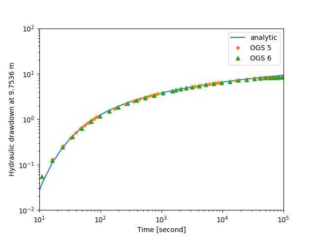
The figure demonstrates a good match between the analytical solution and the numerical solutions obtained using OGS-5 and OGS-6 within the time interval [10, 10$^4$] s, consistent with the results provided in [2] and [3]. A similar good match is observed in the following figure, which compares the head profiles at t=1728 s:

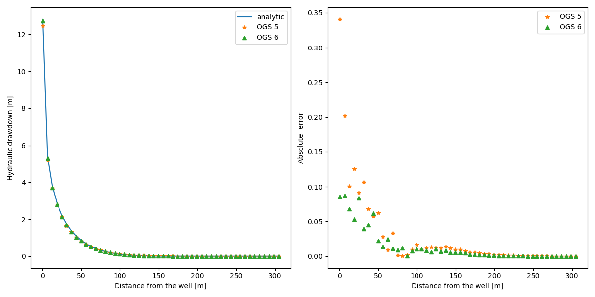At the point with the largest head value, the absolute error of the numerical solution is approximately 0.34.

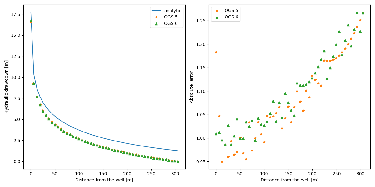
Beyond 10$^4$, an evident discrepancy arises between the analytical solution and the numerical solutions. This discrepancy increases over time due to the inability of the numerical method for a bounded domain (like the FEM) to represent an infinite domain accurately.

The figures below show the comparison of the head profiles at t=10$^5$ s, highlighting this significant discrepancy.

Conclusions

The analytical solutions are obtained for an ideal problem with an infinite domain. However, in the FEM analysis, the infinite domain must be approximated within a finite range. Therefore, the numerical method provides accurate solutions only for positions relatively close to the well and within a specific time interval. Despite this limitation, real-world application are typically constrained by similar conditions, making the numerical approach valid and practical for most idealized cases from the in situ experiments.

Reference

[1] Srivastava, R. and Guzman‐Guzman, A., 1998. Practical approximations of the well function. Groundwater, 36(5), pp.844-848.

[2] Pinder, G.F. and Frind, E.O., 1972. Application of Galerkin’s procedure to aquifer analysis. Water Resources Research, 8(1), pp.108-120.

[3] Kolditz, O., Shao, H., Wang, W. and Bauer, S., 2016. Thermo-hydro-mechanical chemical processes in fractured porous media: modelling and benchmarking (Vol. 25). Berlin: Springer.