Liquid flow with raster parameter based boundary condition

• Parabolic/LiquidFlow/RasterParameter/GroundwaterModelWithRasterBC.prj

Motivation

Specifying spatially and temporally heterogeneous parameters for models with fine mesh resolution and many time steps can lead to very large input files.

For instance, let us assume that the discretization of the study domain contains n elements and that t time steps should be simulated. Hence, you need $n \times t$ storage space.

For instance, sometimes the spatial distribution of the boundary values is given by raster data with a different spatial resolution than the subdomain mesh on which the boundary values are to be set. In such cases, the raster parameter can be used both to reduce the memory footprint of the input data enormously and also to avoid time-consuming preprocessing.

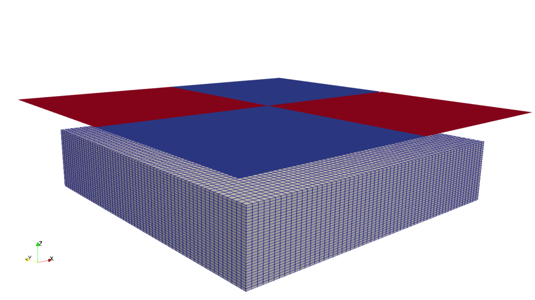
In the figure, the 2x2 raster contains 4 raster cells or 4 (possible different) values. In the example illustration, each raster grid cell covers 225 surface elements. If we were to store this information directly in the surface mesh, we would need about 225 times more memory.

Examples

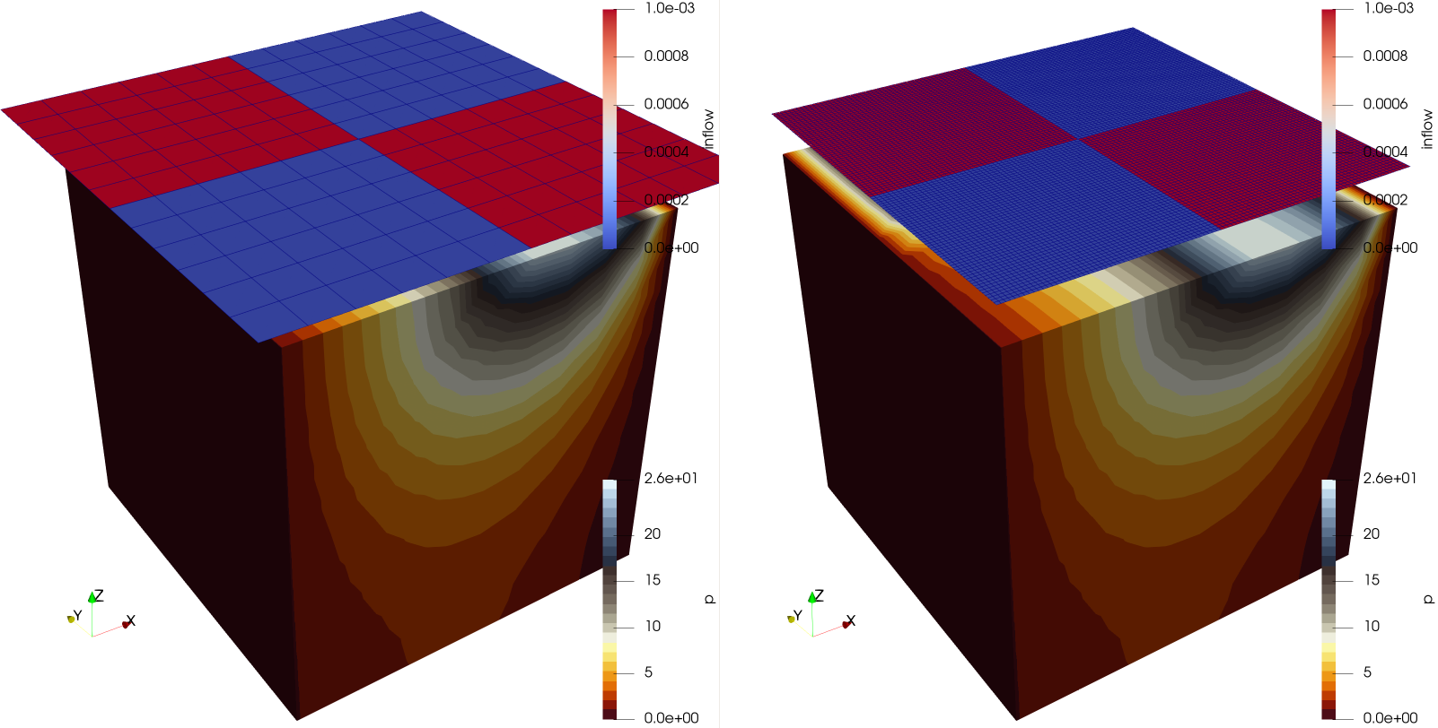
The first simple example should demonstrate the application of a boundary condition based on the raster parameter. We start with homogeneous parabolic problem:

w.r.t boundary conditions

The domain $\Omega = [0,1]^3$ is a cube. Dirichlet-type boundary conditions are set on the left ($x=0$) side and the right ($x=1$) side of the cube. On the top a Neumann-type boundary condition is set by a raster parameter. Here, simulations of two almost identical models are conducted. The only difference is the raster used for setting the boundary condition. The first simulation is done with a coarse raster as input for the boundary condition, the second one is executed with a fine raster as input.

Specification in OGS project file

In the parameter specification section of the project file it is possible to add a parameter type with the type Raster.

Step 1: Loading raster data

<rasters>
    <raster>
        <file>RasterFileName.nc</file>
        <variable>VariableInNetCDFFile</variable>
        <dimenension>DimensionOfVariable</dimension> <!-- optional; default 1 -->
    </raster>
</rasters>

A snippet from a project file looks is:

<rasters>
    <raster>
        <file>recharge_GDM_DE1_1951-2019_monthly_dailymean_mm_per_day_EPSG25832.nc</file>
        <variable>recharge</variable>
        <dimenension>1</dimension>
    </raster>
</rasters>

Step 2: Creating parameter from the loaded raster data

The name of the raster parameter shall be constructed as follows: RasterFileName_VariableInNetCDFFile_DimensionOfVariable

<parameter>
    <name>RasterFileName_VariableInNetCDFFile_DimensionOfVariable</name>
    <type>Raster</type>
</parameter>

The corresponding snippet from a project file would be:

<parameter>
    <name>recharge_GDM_DE1_1951-2019_monthly_dailymean_mm_per_day_EPSG25832_recharge_1</name>
    <type>Raster</type>
</parameter>

Step 3: Using the parameter in boundary condition specification

<boundary_condition>
    <mesh>Subsurface_Top</mesh>
    <type>Neumann</type>
    <parameter>RasterFileName_VariableInNetCDFFile_DimensionOfVariable</parameter>
</boundary_condition>

In an practical example the corresponding XML description of the boundary condition is then:

<boundary_condition>
    <mesh>Subsurface_Top</mesh>
    <type>Neumann</type>
    <parameter>recharge_GDM_DE1_1951-2019_monthly_dailymean_mm_per_day_EPSG25832_recharge_1</parameter>
</boundary_condition>

Results

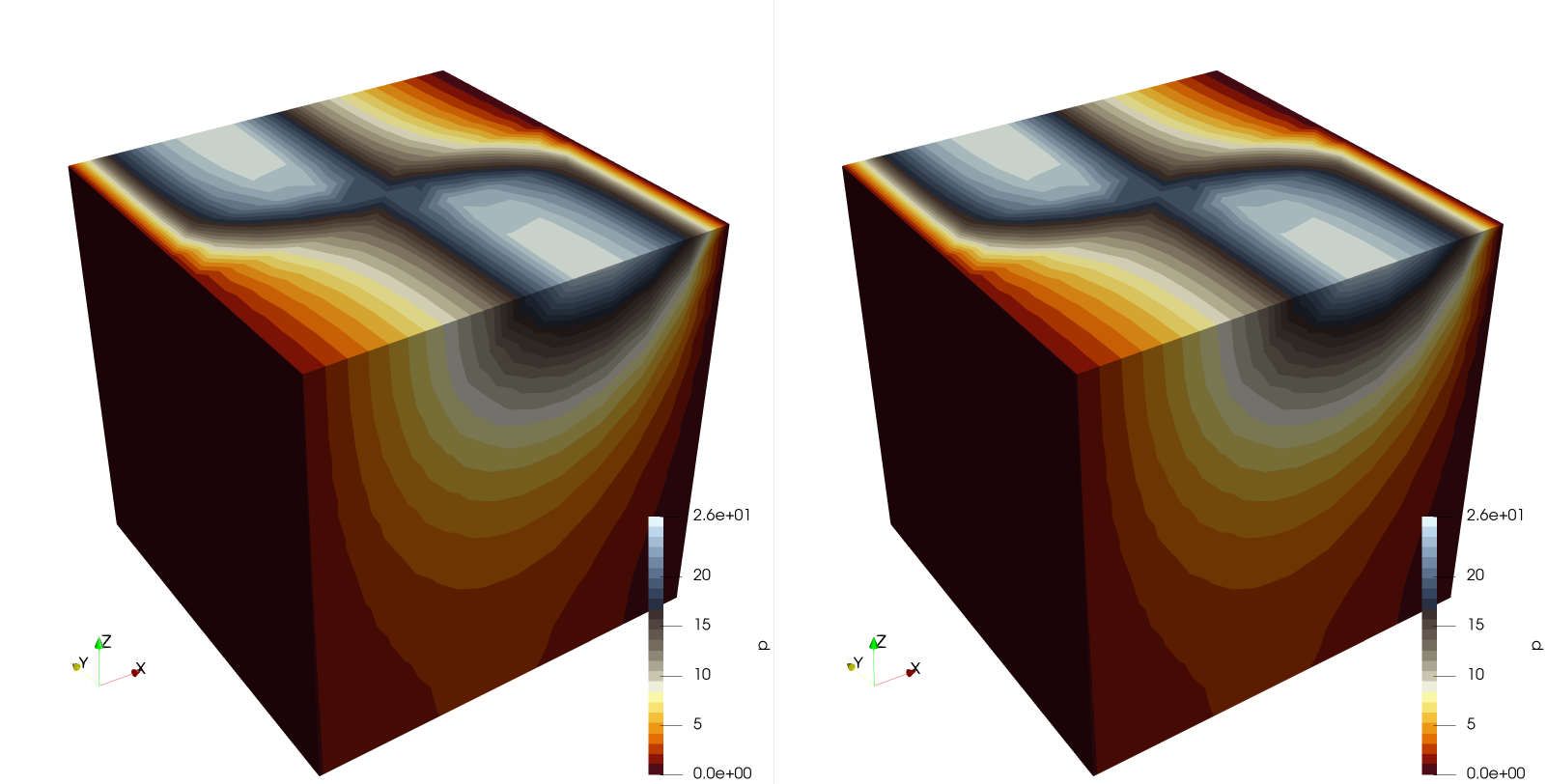
The pressure distribution within the domain is depicted in the following figure (again left: coarse raster input; right: fine raster input). The distributions are identical up to machine precision.