H process: Theis solution (Pumping well)
![]() This page is based on a Jupyter notebook.
This page is based on a Jupyter notebook.


# modules…
(click to toggle)
# modules
import os
import time
from pathlib import Path
from subprocess import run

import matplotlib.pyplot as plt
import matplotlib.tri as tri
import numpy as np
import pyvista as pv
import vtk
import vtuIO
from scipy.special import exp1
from vtk.util.numpy_support import vtk_to_numpy
# settings…
(click to toggle)
# settings
path = "./"
fig_dir = "./figures/"
prj_name = "axisym_theis"
prj_file = f"{prj_name}.prj"
pvd_name = "liquid_pcs"
vtu_name = "axisym_theis.vtu"
title = "H process: Theis solution (Pumping well)"

out_dir = Path(os.environ.get("OGS_TESTRUNNER_OUT_DIR", "_out"))
if not out_dir.exists():
out_dir.mkdir(parents=True)H process: Theis solution
Problem description
Theis` problem examines the transient lowering of the water table induced by a pumping well. The assumptions required by the Theis solution are:
The aquifer
- is homogeneous, isotropic, confined, infinite in radial extent,
- has uniform thickness, horizontal piezometric surface.
The well
- is fully penetrating the entire aquifer thickness,
- has a constant pumping rate,
- well storage effects can be neglected,
- no other wells or long term changes in regional water levels.
Analytical solution
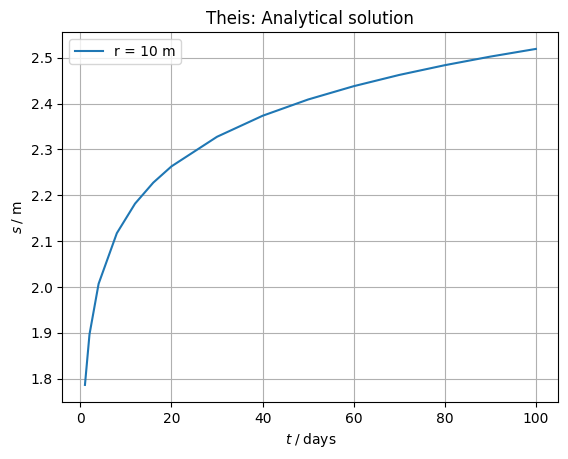
The analytical solution of the drawdown as a function of time and distance is expressed by
$$ s(r,t) = h_0 - h(r,t) = \frac{Q}{4\pi T}W(u), \quad \mathrm{where}\quad u = \frac{r^2S}{4Tt}. $$where
- $s$ [$L$] is the drawdown or change in hydraulic head,
- $h_0$ is the constant initial hydraulic head,
- $h$ is the hydrauic head at distance $r$ at time $t$
- $Q$ [$L^3T^{-1}$] is the constant pumping (discharge) rate
- $S$ [$-$] is the aquifer storage coefficient (volume of water released per unit decrease in $h$ per unit area)
- $T$ [$L^2T^{-1}$] is the transmissivity (a measure of how much water is transported horizontally per unit time).
The Well Function, $W(u)$ is the exponential integral, $E_1(u).$ $W(u)$ is defined by an infinite series:
$$ W(u) = - \gamma - \ln u + \sum_{k=1}^\infty \frac{(-1)^{k+1} u^k}{k \cdot k!} $$where
- $\gamma=0.577215664$ is the Euler-Mascheroni constant
For practical applications an approximation to the exponential integral is used often:
$$W(u) \approx -\gamma - \ln u$$This results in an expression for $s(r,t)$ known as the Jacob equation:
$$ s(r,t) = -\frac{Q}{4\pi T}\left(\gamma + \ln u \right). $$For more details we refer to Srivastava and Guzman-Guzman (1998).
# source: https://scipython.com/blog/linear-and-non-linear-fitting-of-the-theis-equation/…
(click to toggle)
# source: https://scipython.com/blog/linear-and-non-linear-fitting-of-the-theis-equation/


def calc_u(r, S, T, t):
    """Calculate and return the dimensionless time parameter, u."""

    return r**2 * S / 4 / T / t


def theis_drawdown(t, S, T, Q, r):
    """Calculate and return the drawdown s(r,t) for parameters S, T.

    This version uses the Theis equation, s(r,t) = Q * W(u) / (4.pi.T),
    where W(u) is the Well function for u = Sr^2 / (4Tt).
    S is the aquifer storage coefficient,
    T is the transmissivity (m2/day),
    r is the distance from the well (m), and
    Q is the pumping rate (m3/day).

    """

    u = calc_u(r, S, T, t)
    return Q / 4 / np.pi / T * exp1(u)
Q = 2000 # Pumping rate from well (m3/day)…
(click to toggle)
Q = 2000  # Pumping rate from well (m3/day)
r = 10  # Distance from well (m)

# Time grid, days.
t = np.array([1, 2, 4, 8, 12, 16, 20, 30, 40, 50, 60, 70, 80, 90, 100])

# Calculate some synthetic data to fit.
S, T = 0.0003, 1000
s = theis_drawdown(t, S, T, Q, r)

# Plot the data
titlestring = "Theis: Analytical solution"
plt.title(titlestring)
plt.plot(t, s, label="r = " + str(r) + " m")
plt.xlabel(r"$t\;/\;\mathrm{days}$")
plt.ylabel(r"$s\;/\;\mathrm{m}$")
plt.legend()
plt.grid()
plt.show()
# Recalculation from days in sec…
(click to toggle)
# Recalculation from days in sec
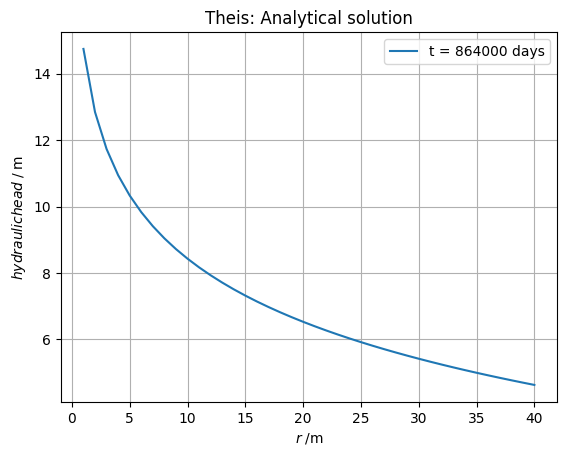
Q = 0.016 # Pumping rate from well (m3/s)
t = 864000 # Time in s.
# Distance from well (m)
##r = np.array([0.5, 1, 2, 4, 8, 12, 16, 20, 25, 30, 35, 40])
r = np.arange(1, 41, 1)
##print(r)
# Calculate some synthetic data to fit.
S = 0.001
T = 9.2903e-4
u = calc_u(r, S, T, t)
s = theis_drawdown(t, S, T, Q, r)
s = s - 5 # reference head
# Plot the data
titlestring = "Theis: Analytical solution"
plt.title(titlestring)
plt.plot(r, s, label="t = " + str(t) + " days")
plt.xlabel(r"$r\;/\mathrm{m}$")
plt.ylabel(r"$hydraulic head\;/\;\mathrm{m}$")
plt.legend()
plt.grid()
plt.show()
Numerical solution
mesh = pv.read(vtu_name)…
(click to toggle)
mesh = pv.read(vtu_name)
print("inspecting vtu-file")
print(mesh)inspecting vtu-file
UnstructuredGrid (0x7b75f578e1a0)
N Cells: 354
N Points: 476
X Bounds: 3.048e-01, 3.048e+02
Y Bounds: 0.000e+00, 1.000e+00
Z Bounds: 0.000e+00, 0.000e+00
N Arrays: 1
print("inspecting mesh and initial conditions")…
(click to toggle)
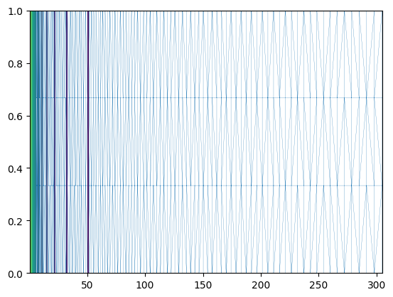
print("inspecting mesh and initial conditions")
# file
reader = vtk.vtkXMLUnstructuredGridReader()
reader.SetFileName(vtu_name)
reader.Update()  # Needed because of GetScalarRange
data = reader.GetOutput()
pressure = data.GetPointData().GetArray("OGS5_pressure")
# points
points = data.GetPoints()
npts = points.GetNumberOfPoints()
x = vtk_to_numpy(points.GetData())
triang = tri.Triangulation(x[:, 0], x[:, 1])
# plt.triplot(triang, 'go-', lw=1.0)
plt.triplot(triang, lw=0.2)
plt.tricontour(triang, pressure, 16)inspecting mesh and initial conditions
<matplotlib.tri._tricontour.TriContourSet at 0x7b75f5861670>
Running OGS
# run ogs…
(click to toggle)
# run ogs
t0 = time.time()
print("run ogs")
print(f"ogs {prj_file} > log.txt")
run(f"ogs {prj_file} -o {out_dir} > {out_dir}/log.txt", shell=True, check=True)
tf = time.time()
print("computation time: ", round(tf - t0, 2), " s.")run ogs
ogs axisym_theis.prj > log.txt
computation time: 0.46 s.
Spatial Profiles
# Read simulation results…
(click to toggle)
# Read simulation results
pvdfile = vtuIO.PVDIO(f"{out_dir}/{pvd_name}.pvd", dim=2)
xaxis = [(i, 0, 0) for i in np.linspace(start=1.0, stop=40, num=40)]
r_x = np.array(xaxis)[:, 0]
time = [8.64, 86.4, 1728, 24192, 172800, 604800, 864000]
pressure_xaxis_t = pvdfile.read_set_data(
t, "OGS5_pressure", data_type="point", pointsetarray=xaxis
)
plt.plot(r_x, pressure_xaxis_t, "x", label="OGS5, t = 1728 sec")
for t in time:
pressure_xaxis_t = pvdfile.read_set_data(
t, "pressure", data_type="point", pointsetarray=xaxis
)
plt.plot(r_x, pressure_xaxis_t, label="t = " + str(t) + " sec")
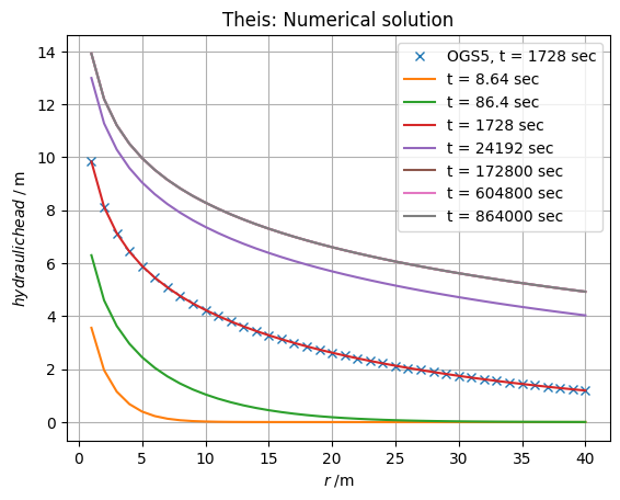
titlestring = "Theis: Numerical solution"
plt.title(titlestring)
plt.xlabel(r"$r\;/\mathrm{m}$")
plt.ylabel(r"$hydraulic head\;/\;\mathrm{m}$")
plt.legend()
plt.grid()
# plt.savefig("theis.png")
plt.show()
time = [864000]…
(click to toggle)
time = [864000]
pressure_xaxis_t = pvdfile.read_set_data(
t, "pressure", data_type="point", pointsetarray=xaxis
)
# plot configuration
##plt.rcParams['figure.figsize'] = (16, 6)
##plt.rcParams['font.size'] = 12
##fig1, (ax1, ax2) = plt.subplots(1, 2)
fig, ax = plt.subplots(ncols=2, figsize=(12, 4))
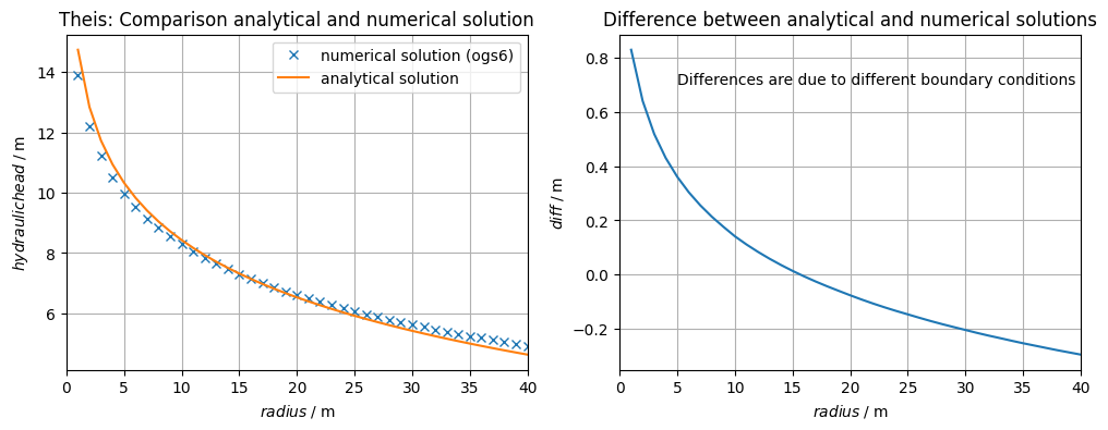
titlestring = "Theis: Comparison analytical and numerical solution"
ax[0].set_title(titlestring)
ax[0].set_xlim(0, 40)
ax[0].plot(r_x, pressure_xaxis_t, "x", label="numerical solution (ogs6)")
ax[0].plot(r, s, label="analytical solution")
ax[0].set_xlabel(r"$radius\;/\;\mathrm{m}$")
ax[0].set_ylabel(r"$hydraulic head\;/\;\mathrm{m}$")
ax[0].grid()
ax[0].legend()
##diff = np.setdiff1d(s,pressure_xaxis_t,assume_unique=False)
##print(diff)
titlestring = "Difference between analytical and numerical solutions"
caption = "Differences are due to different boundary conditions"
ax[1].set_title(titlestring)
ax[1].set_xlim(0, 40)
ax[1].plot(r, s - pressure_xaxis_t, label="")
ax[1].set_xlabel(r"$radius\;/\;\mathrm{m}$")
ax[1].set_ylabel(r"$diff\;/\;\mathrm{m}$")
ax[1].grid()
ax[1].text(5, 0.7, caption, ha="left")
##plt.savefig("theis-ana+num.png")
plt.show()
OGS links
- description: https://www.opengeosys.org/docs/benchmarks/
- project file: https://gitlab.opengeosys.org/ogs/ogs/-/blob/master/Tests/Data/Parabolic/LiquidFlow/AxiSymTheis/axisym_theis.prj
References
- Rajesh Srivastava and Amado Guzman-Guzman (1998): Practical Approximations of the Well Function. Groundwater, 36(5): 844-848, https://doi.org/10.1111/j.1745-6584.1998.tb02203.x
Credits
- Christian for the analytical solution in Python, https://scipython.com/blog/linear-and-non-linear-fitting-of-the-theis-equation/
- Wenqing Wang for set-up the OGS benchmark, https://www.opengeosys.org/docs/benchmarks/liquid-flow/liquid-flow-theis-problem/
- Jörg Buchwald for ogs6py (now part of ogstools) and VTUInterface, https://joss.theoj.org/papers/6ddcac13634c6373e6e808952fdf4abc
This article was written by Wenqing Wang, Olaf Kolditz. If you are missing something or you find an error please let us know.
Generated with Hugo 0.147.9
in CI job 577984
|
Last revision: August 24, 2022