Buildup Test

• /Parabolic/LiquidFlow/BuildupTest/buildup_test.prj

Problem description

The pressure buildup test is performed by shutting in a producing well at time $t=t_p$, after which a smooth rise of the well head pressure can be observed. For a geothermal reservoir, the buildup test result is interpreted using a Horner plot in order to evaluate the reservoir permeability or transmissivity. In this benchmark, observation data from a geothermal well is employed to parameterize the numerical model. In the model, a time dependent nodal source term was set up to represent the shut-in operation. The simulated pressure profile is then verified against the analytical solution.

Model Setup

This benchmark represents a scenario in which the well had been producing geothermal brine for $118\ \mathrm{h}$ at a rate of $78\ t/\mathrm{h}$ and was then shut in for a buildup test. At the given reservoir temperature (260$^\circ$C) and pressure ($47\ \mathrm{bar}$), the density and viscosity of the water and steam mixture were calculated as $\rho=78.68\ \mathrm{kg/m^3}$ and $\mu=1.295\times10^{-4}\ \mathrm{Pa\ s}$. The compressibility of the mixture was estimated as $nc_t=0.0805\ \mathrm{bar^{-1}}$ ($n$ refers to the porosity of the reservoir), which yields a specific storage coefficient of $S=\rho gnc_t=6.21\times 10^{-4}\ \mathrm{m^{-1}}$. The observed pressure readings during the buildup test are cited from Chapter 6 of the book Geothermal Power Generation [1], and the data is archived in the Appendix.

The permeability of the reservoir can be estimated by means of a Horner plot, in which the pressure $p$ is plotted against $(t_p+\Delta t)/\Delta t$, i.e. Horner time on a semi-logarithmic scale (cf. Figure 1). In the Horner plot, the data points form a straight line in the late-time period of the test. Note that the time increases in the opposite direction of the X-axis. Therefore, the linear section appears at the left side of the diagram.

\centering

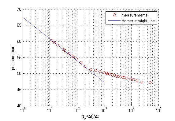
Figure 1: Horner plot ($p$ vs $(t_p+\Delta t)/\Delta t$) for buildup test showing the inferred Horner straight line

The slope $m$ of the Horner straight line is expressed as:

$$m=0.1832\frac{Q\mu}{\kappa b}$$

in which $Q\ \mathrm{[L^3/T]}\ (Q>0)$ is the production rate of the well before shut-in, $\kappa\ \mathrm{[L^2]}$ is the permeability and $b\ \mathrm{[L]}$ is the aquifer thickness. From the Horner plot, we can infer a Horner straight line with a slope of $m=0.79$. Therefore the transmissivity of the aquifer can be calculated as

$$\begin{aligned} \kappa b&=&0.1832\frac{Q\mu}{m}=0.1832\frac{((78000/3600)/78.68)\times1.295\times10^{-4}}{7.09\times10^5}\\&=&9.2\times10^{-12}\ \mathrm{m^3}\end{aligned}$$

In addition, the straight line in the Horner plot can be extracted to a Horner time of 1, which corresponds to the infinite shut-in time $(\Delta t)$. This leads to an extrapolated pressure $p_0$ of $67.5~\mathrm{kPa}$, which is the undisturbed reservoir pressure .

Input files

The benchmark project is defined in the input file buildup_test.prj. It defines the process to be solved as “LiquidFlow” and the primary variable is hence pressure. The initial condition is set to $p_0=67.5\ \mathrm{bar}$ and the undisturbed boundary is achieved by a large domain size $(r=1000\ \mathrm{m})$. The time-dependent source term is applied in this benchmark. From the beginning until $t=424800$ sec, the pumping rate was maintained at a constant rate. Afterwards, the well is shut-in and pressure starts to build up. The geometries used to specify the model domain, boundary conditions, and source term can be found in line_1000_axi.gml file. The mesh is specified in line_1000_axi.vtu, which is stored in the VTK format and can be directly visualized in ParaView.

Analytical solution

The pressure buildup test is comparable to a pumping recovery test as the extraction rate is first kept constant at $Q$, and then becomes zero at $t=t_p$. This benchmark then adopts the same assumptions as in the Theis' problem. The analytical solution of the pressure difference $\Delta p$ with respect to the initial pressure $p_0$ is the sum of two Theis curves: one starting at $t=0$ and another starting at $t=t_p$ but with an opposite extraction rate, i.e. for $t\leq t_p$,

$$\Delta p=\rho g \frac{-Q}{4\pi T}W\left(\frac{r^2S}{4Tt}\right)$$

and for $t>t_p$,

$$\Delta p=\rho g \frac{-Q}{4\pi T}W\left(\frac{r^2S}{4Tt}\right)+\rho g \frac{Q}{4\pi T}W\left(\frac{r^2S}{4T(t-t_p)}\right)$$

Results and evaluation

The pressure evolution is simulated throughout the domain and the result is compared with the analytical solution at $r=10.287\ \mathrm{m}$. In Figure 2, it can be observed that the numerical model fits with the analytical solution very well. The absolute and relative error between the analytical and numerical solution is depicted in Figure 3.

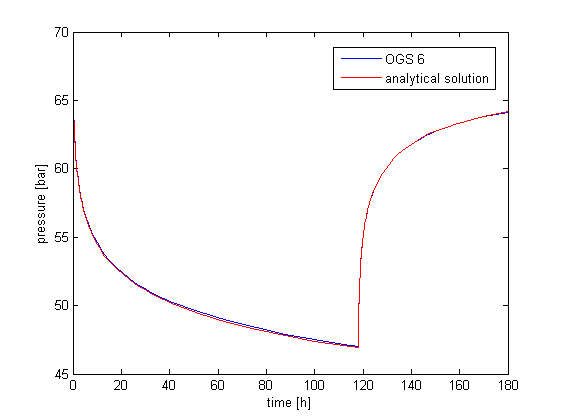
Figure 2: OGS 6 result compared with analytical solution

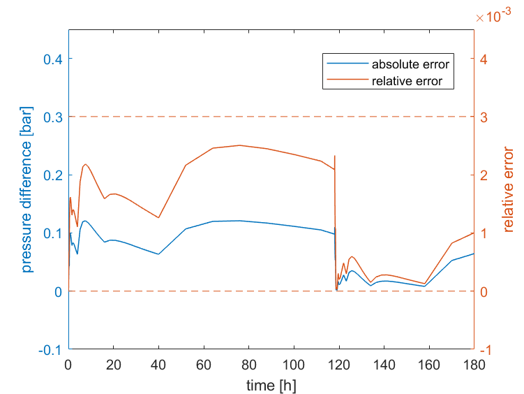
Figure 3: Absolute and relative error

References

[1] RN Horne. Characterization, evaluation, and interpretation of well data. In: R DiPippo, editor,Geothermal Power Generation, chapter 6, pages 141–163.Elsevier, 2016.

Appendix

\centering

$\Delta t$ (h)	$\Delta p$ (bar)	$\Delta t$ (h)	$\Delta p$ (bar)
0.0024	0.174	0.1708	3.65
0.0073	0.695	0.2442	4.00
0.0098	1.13	0.3667	4.26
0.0122	1.30	0.6111	5.13
0.0171	1.57	0.8556	6.35
0.022	1.74	1.2194	7.48
0.0244	1.91	1.5861	8.17
0.0292	2.00	1.8361	8.43
0.0367	2.09	2.4417	9.22
0.0414	2.17	3.4167	10.2
0.0489	2.43	3.8611	10.4
0.0586	2.61	6.3056	11.8
0.0733	2.78	8.3056	12.6
0.0856	2.96	10.9722	13.2
0.0975	3.13

: Pressure measurements during well buildup[]{label=“table:1”}