Seabed response to water waves, FEniCSx – OGS comparison
![]() This page is based on a Jupyter notebook.
This page is based on a Jupyter notebook.


 |
|---|
Seabed response to water waves
In this benchmark example, the response of a seabed to water waves is determined by the application of the theory of poroelasticity. The seabed is described as a homogeneous poroelastic medium consisting of a solid phase (i.e. sand grains) and pores that are quasi-saturated with a Newtonian fluid, such as water. The pores are not completely saturated with water as they contain small bubbles of air, which cause the compressibility of the pore space. The pressure along the bottom of the sea depends on the water level and therefore varies according to the water waves in space as well as time. Arnold Verruijt in his book “Theory and problems of poroelasticity” [1] derives an analytical solution of the stress distribution in the seabed for the case of sinusoidal water waves. For the analytical solution, some assumptions have been made:
- disregarded body forces
- homogenous linear elastic material
- compressibility of the particles is taken into account
- water waves are stationary and only dependent on one horizontal direction (x-direction in this example)
- plain strain condition
The last two assumptions allow a simplification of the three-dimensional seabed to a planar geometry.
For verification of the numerical model, Arnold Verruijt’s analytical solution will be compared to the results of the numerical calculation. The behaviour of the seabed depends on various parameters describing the soil, fluid and wave properies. In this example, the parameters of both the analytical and the numerical solution are chosen as follows:
Input parameters
$$ \begin{aligned} &\begin{array}{llll} C_{f} & \textsf{compressibility of the fluid} & \textsf{[1/Pa]} & C_{f} = 0\,\textsf{Pa}^{-1}\\ C_{s} & \textsf{compressibility of the solid particles}& \textsf{[1/Pa]} & C_{s} = 0\,\textsf{Pa}^{-1}\\ G & \textsf{shear modulus} & \textsf{[Pa]} & G = 100\, \textsf{kPa} \\ K & \textsf{bulk modulus} & \textsf{[Pa]} & K = \frac{2}{3} G \ (\textsf{with } \nu = 0) \\ L & \textsf{wave length} & \textsf{[m]} & L = 100 \textsf{ m} \\ T & \textsf{periodic time} & \textsf{[s]} & T=\frac{1}{f} = 10\,\textsf{s} \\ \gamma_{w} & \textsf{volumetric weight of water} & \textsf{[kN/m³]} & \gamma_{w} = 9,81\,\textsf{kN/m³} \\ \kappa & \textsf{(intrinsic) permeability} & \textsf{[m²]} & \kappa = 10^{-11}\,\textsf{m² } ( \textsf{equals } k_{f}=10^{-4} \textsf{ m/s} ) \\ \mu & \textsf{dynamic viscosity of water} & \textsf{[Pa s]} & \mu = 1.3\,\textsf{mPa s } ( \textsf{at } \theta=10\,\textsf{°C}) \\ \nu & \textsf{Poisson's ratio} & \textsf{[-]} & \nu = 0\\ \end{array} \end{aligned} $$Derived parameters
$$ \begin{aligned} &\begin{array}{llll} c_{v} & \textsf{coefficient of consolidation} & \textsf{[m²/s]} & c_{v} = \frac{kG(1+m)}{(1+SG(1+m))\gamma_{w}} = \frac{k(K+\frac{4}{3}G)}{(1+S(K+\frac{4}{3}G))\gamma_{w}} \\ m & \textsf{dimensionless parameter} & \textsf{[-]} & m = \frac{1}{1-2\nu} = \frac{K+\frac{1}{3}G}{G} \\ k & \textsf{hydraulic conductivity} & \textsf{[m/s]} & k = \frac{\kappa\rho_{f}g}{\mu} \\ C_{m} & \textsf{compressibility of the porous medium} & \textsf{[1/Pa]}& C_{m} = \frac{1}{K} \\ S & \textsf{storativity of the pore space}& \textsf{[-]} & S=nC_{f}+(\alpha-n)C_{s} \\ \alpha & \textsf{Biot coefficient} & \textsf{[-]} & \alpha=1-\frac{C_{s}}{C_{m}} \\ \lambda & \textsf{wave number} & \textsf{[1/m]} & \lambda=\frac{\omega}{c} = \frac{\omega T}{L} \\ \xi^2 & \textsf{complex parameter} & \textsf{[1/m²]} & \xi^2 = \lambda^2 + \frac{\omega}{c_{v}}i \\ \omega & \textsf{frequency of the wave} & \textsf{[1/s]} & \omega = 2 \pi f \\ \end{array} \end{aligned} $$Analytical solution for stationary waves
Boundary conditions
The considered region is the half plane $y>0$ with a load in the form of a stationary wave applied on the surface $y=0$. The boundary conditions at $y=0$ are:
$$ \begin{align} p&=\tilde{p}\cdot e^{i(\omega t-\frac{\pi}{2})}\cdot\cos(\lambda x) \\ \sigma'_{yy}&=0 \\ \sigma'_{xy}&=0 \end{align} $$where $p$ is the pore pressure, $\tilde{p}$ is the amplitude of the applied load, $\sigma'_{yy}$ is the effective vertical stress and $\sigma'_{xy}$ is the effective shear stress. The boundary condition of the pore pressure describes the space- and time-dependent water wave. Compared to Arnold Verruijt’s solution, in this example there is a phase shift of $-\frac{\pi}{2}$ in the time-dependent part. The phase shift is necessary to obtain a water wave that starts oszillating from the equilibrium state (sine instead of cosine) and thus to be able to set an initial condition of $p=0$ Pa on the whole domain in the numerical solution.
With these boundary conditions, the following four constants are determined:
$$ \begin{align} B_{1} &= (1+m)(\xi^2-\lambda^2)-2\lambda(\xi-\lambda) \\ B_{2} &= 2m\theta\lambda\xi+\theta[(1+m)(\xi^2-\lambda^2)-2\lambda(\xi-\lambda)] \\ B_{3} &= 2m\theta\lambda\\ D &= 2\lambda[2\lambda(\xi-\lambda)-(1+m)(1+m\theta)(\xi^2-\lambda^2)] \end{align} $$The stresses
For the given boundary conditions, the pore pressure and the effective stresses can be calculated with the following equations. According to the sign convention commonly used in soil mechanics, compressive stresses are positive and tensile stresses are negative. In all these equations, the real part is to be taken only.
$$ \begin{align} \frac{p}{\tilde{p}} &= \mathscr{R}\left\{\frac{-2\lambda B_{1}\cdot e^{-\lambda y}-(1+m)(\xi^2-\lambda^2)B_{3}\cdot e^{-\xi y}}{D}\cdot e^{i(\omega t-\frac{\pi}{2})}\cdot\cos(\lambda x)\right\} \\ \\ \frac{\sigma'_{xx}}{\alpha\tilde{p}} &= \mathscr{R}\left\{\frac{[-2(m-1)\lambda\theta+2\lambda(1+m\theta)\lambda y]B_{1}\cdot e^{-\lambda y}-2\lambda B_{2} \cdot e^{-\lambda y}+[(m-1)(\xi^2-\lambda^2)-2\lambda^2]B_{3} \cdot e^{-\xi y}}{D} \cdot e^{i(\omega t-\frac{\pi}{2})} \cdot \cos(\lambda x) \right\} \\ \\ \frac{\sigma'_{yy}}{\alpha\tilde{p}} &= \mathscr{R}\left\{\frac{[-2(m+1)\lambda\theta-2\lambda(1+m\theta)\lambda y]B_{1}\cdot e^{-\lambda y}+2\lambda B_{2} \cdot e^{-\lambda y}+[(m-1)(\xi^2-\lambda^2)+2\xi^2]B_{3} \cdot e^{-\xi y}}{D} \cdot e^{i(\omega t-\frac{\pi}{2})} \cdot \cos(\lambda x) \right\} \\ \\ \frac{\sigma'_{xy}}{\alpha\tilde{p}} &= \mathscr{R}\left\{\frac{[-2\lambda(1+m\theta)\lambda y-2\lambda\theta]B_{1}\cdot e^{-\lambda y}+2\lambda B_{2} \cdot e^{-\lambda y}+2\xi\lambda B_{3} \cdot e^{-\xi y}}{D} \cdot e^{i(\omega t-\frac{\pi}{2})} \cdot \sin(\lambda x) \right\} \\ \end{align} $$
import os…
(click to toggle)
import os
import subprocess
from pathlib import Path

import gmsh
import matplotlib.patches as mpatches
import matplotlib.pyplot as plt
import meshio
import numpy as np
import ogstools as ot
import pyvista as pv
plt.rcParams.update({"font.size": 12})…
(click to toggle)
plt.rcParams.update({"font.size": 12})
plt.rcParams["lines.linestyle"] = "-"
plt.rcParams["lines.markersize"] = 10
plt.rcParams["xtick.labelsize"] = 12
plt.rcParams["ytick.labelsize"] = 12
plt.rcParams["axes.titlesize"] = 12
plt.rcParams["axes.labelsize"] = 12

pv.set_plot_theme("document")
pv.set_jupyter_backend("static")
def compute_pressure_and_stresses(t, x, z):…
(click to toggle)
def compute_pressure_and_stresses(t, x, z):
    n = 0.4
    G = 100e3  # [Pa]
    K = 2 / 3 * G  # [Pa]    (with ny=0)
    ny = 0  # E = 3K(1-2ny) = 2G(1+ny)
    Cf = 0  # in the book: Cf = 0.001/K
    Cs = 0
    Cm = 1 / K
    my = 1.3e-3  # [Pa*s]
    kappa = 1e-11  # [m²]    (medium sand, kf=10e-4 m/s)
    gamma_w = 9.81e3  # [Pa/m]
    lam = 2 * np.pi * 0.1 * 10 / 100
    omega = 2 * np.pi * 0.1

    k = kappa * gamma_w / my  # Gl. (1.33)
    alpha = 1 - Cs / Cm  # Gl. (4.15)
    S = n * Cf + (alpha - n) * Cs  # Gl. (1.28)
    theta = S * G / alpha**2  # Gl. (4.13)
    m = 1 / (1 - 2 * ny)  # = K+1/3*G/G                               # Gl. (4.5)
    cv = k * G * (1 + m) / (alpha**2 * (1 + theta + m * theta) * gamma_w)  # Gl. (4.12)
    xi_2 = complex(lam**2, (omega / cv))  # Gl. (4.19)

    B1 = (1 + m) * (xi_2 - lam**2) - 2 * lam * (np.sqrt(xi_2) - lam)
    B2 = 2 * m * theta * lam * np.sqrt(xi_2) + theta * (
        (1 + m) * (xi_2 - lam**2) - 2 * lam * (np.sqrt(xi_2) - lam)
    )
    B3 = 2 * m * theta * lam
    D = (
        2
        * lam
        * (
            2 * lam * (np.sqrt(xi_2) - lam)
            - (1 + m) * (1 + m * theta) * (xi_2 - lam**2)
        )
    )
    p_rel = np.real(
        (
            -2 * lam * B1 * np.exp(-lam * z)
            - (1 + m) * (xi_2 - lam**2) * B3 * np.exp(-np.sqrt(xi_2) * z)
        )
        / D
        * np.exp((omega * t - np.pi * 0.5) * 1j)
        * np.cos(lam * x)
    )
    sig_xx_rel = np.real(
        (
            (-2 * (m - 1) * lam * theta + 2 * lam * (1 + m * theta) * lam * z)
            * B1
            * np.exp(-lam * z)
            - 2 * lam * B2 * np.exp(-lam * z)
            + ((m - 1) * (xi_2 - lam**2) - 2 * lam**2) * B3 * np.exp(-np.sqrt(xi_2) * z)
        )
        / D
        * np.exp((omega * t - np.pi * 0.5) * 1j)
        * np.cos(lam * x)
    )
    sig_zz_rel = np.real(
        (
            (-2 * (m + 1) * lam * theta - 2 * lam * (1 + m * theta) * lam * z)
            * B1
            * np.exp(-lam * z)
            + 2 * lam * B2 * np.exp(-lam * z)
            + ((m - 1) * (xi_2 - lam**2) + 2 * xi_2) * B3 * np.exp(-np.sqrt(xi_2) * z)
        )
        / D
        * np.exp((omega * t - np.pi * 0.5) * 1j)
        * np.cos(lam * x)
    )
    sig_xz_rel = np.real(
        (
            (-2 * lam * (1 + m * theta) * lam * z - 2 * lam * theta)
            * B1
            * np.exp(-lam * z)
            + 2 * lam * B2 * np.exp(-lam * z)
            + 2 * np.sqrt(xi_2) * lam * B3 * np.exp(-np.sqrt(xi_2) * z)
        )
        / D
        * np.exp((omega * t - np.pi * 0.5) * 1j)
        * np.sin(lam * x)
    )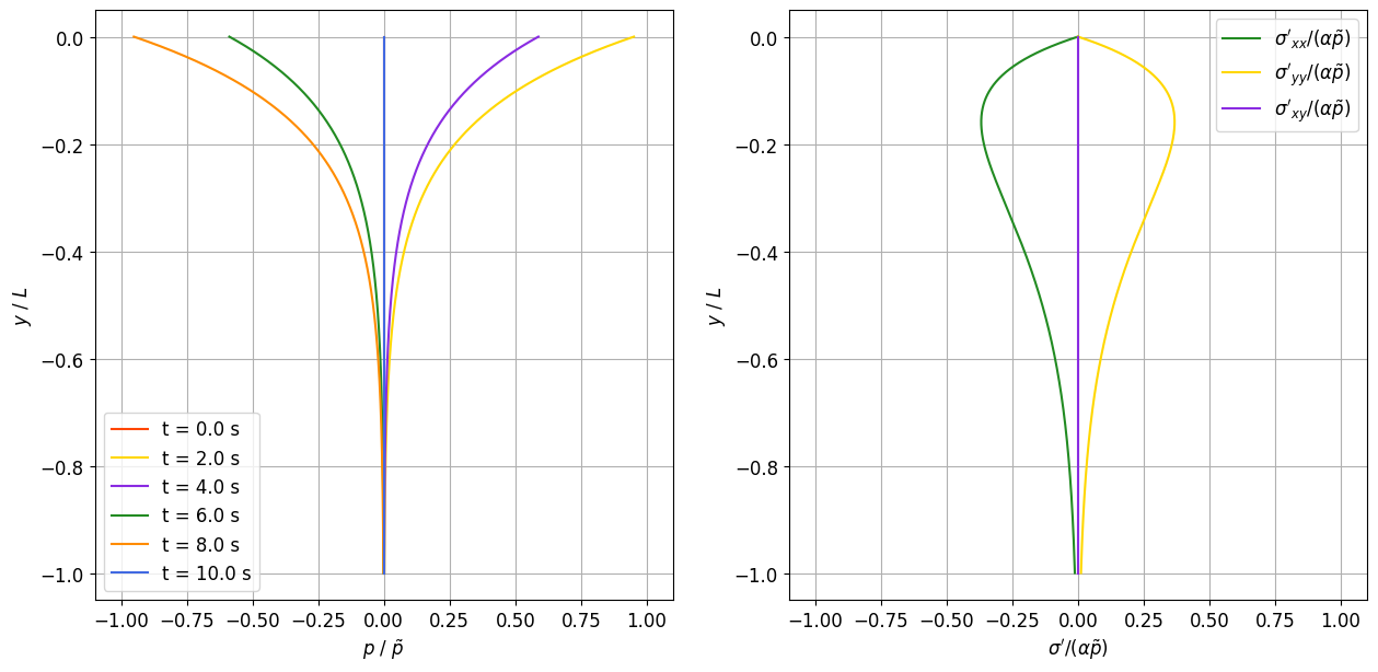
return p_rel, sig_xx_rel, sig_zz_rel, sig_xz_relBy evaluating these equations at different times $t$ and depths $y$, we gain a better understanding of the pressure and stress distribution in the seabed. The below plot illustrates the pore pressure and the amplitude of the effective stresses as a function of depth directly underneath an anti-node of the standing water wave (the place where the amplitude is at maximum, i.e. for $x = k \cdot \frac{L}{2}$, where $k=0, 1, 2,$ …).
Along the top edge of the seabed, the pore pressure is always as large as the applied load and the effective stresses are zero. This means, that all the change in pressure is absorbed by the fluid while the soil particles remain in their initial stress state (in this case zero, since body forces are being disregarded). The increased pore pressure at the top edge cannot propagate freely downwards into the seabed because seepage is limited by the hydraulic conductivity of the soil. Consequently, the pore pressure decreases with depth as the soil matrix gradually takes up the remaining share of the total stress in the seabed.
y = np.linspace(0, 100, 1000)…
(click to toggle)
y = np.linspace(0, 100, 1000)
y_rel = y / 100
colors = {
    0: "orangered",
    2: "gold",
    4: "blueviolet",
    6: "forestgreen",
    8: "darkorange",
    10: "royalblue",
}

fig, ax = plt.subplots(ncols=2, figsize=(15, 7))
for idx in (0, 1):
    ax[idx].grid(True)
    ax[idx].set_ylabel("$y$ / $L$")
    ax[idx].set_xlim(-1.1, 1.1)

for t in [0, 2, 4, 6, 8, 10]:
    ax[0].plot(
        compute_pressure_and_stresses(t, 0, y)[0],
        -y_rel,
        color=colors[t],
        label=f"t = {t:.1f} s",
    )

t = 2.5
ax[0].set_xlabel("$p$ / $\\tilde{p}$")
ax[0].legend()
ax[1].plot(
    compute_pressure_and_stresses(t, 0, y)[1],
    -y_rel,
    color=colors[6],
    label=r"$\sigma'_{xx}/(\alpha\tilde{p})$",
)
# ax[1].plot(compute_pressure_and_stresses(t,0,y)[1]+compute_pressure_and_stresses(t,0,y)[0], -y_rel, linestyle = "--", color = colors[3], label = "$\\sigma_{xx}$/$\\alpha\\tilde{p}$")  # Total horizontal stress
ax[1].plot(
    compute_pressure_and_stresses(t, 0, y)[2],
    -y_rel,
    color=colors[2],
    label=r"$\sigma'_{yy}/(\alpha\tilde{p})$",
)
# ax[1].plot(compute_pressure_and_stresses(t,0,y)[2]+compute_pressure_and_stresses(t,0,y)[0], -y_rel, linestyle = "--", color = colors[1], label = "$\\sigma_{yy}$/$\\alpha\\tilde{p}$")  # Total vertical stress
ax[1].plot(
    compute_pressure_and_stresses(t, 0, y)[3],
    -y_rel,
    color=colors[4],
    label=r"$\sigma'_{xy}/(\alpha\tilde{p})$",
)
ax[1].set_xlabel(r"$\sigma'/(\alpha\tilde{p})$")
ax[1].legend()<matplotlib.legend.Legend at 0x7fcaa74c7a10>
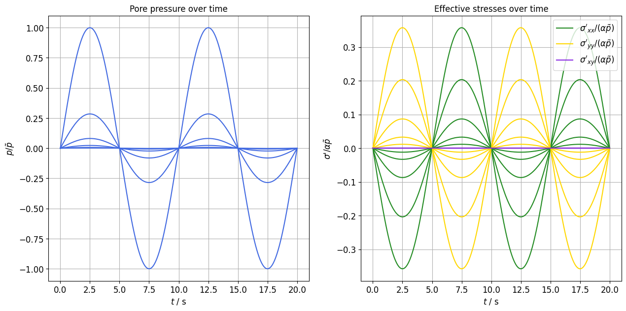
The following plot illustrates the pore pressure and the effective stresses at different depths underneath an anti-node over time. Here it becomes clear that the vertical and the horizontal effective stresses behave symmetrically in space as well as time.
t = np.linspace(0, 20, 200)…
(click to toggle)
t = np.linspace(0, 20, 200)
colors = {1: "gold", 2: "blueviolet", 3: "forestgreen", 4: "royalblue"}

fig, ax = plt.subplots(ncols=2, figsize=(15, 7))
for idx in (0, 1):
    ax[idx].grid(True)
    ax[idx].set_xlabel("$t$ / s")

for y in np.linspace(0, 100, 6):
    ax[0].plot(t, compute_pressure_and_stresses(t, 0, y)[0], color=colors[4])
    ax[0].set_ylabel("$p/\\tilde{p}$")
    ax[1].plot(
        t,
        compute_pressure_and_stresses(t, 0, y)[1],
        color=colors[3],
        label=r"$\sigma'_{xx}/(\alpha\tilde{p})$",
    )
    ax[1].plot(
        t,
        compute_pressure_and_stresses(t, 0, y)[2],
        color=colors[1],
        label=r"$\sigma'_{yy}/(\alpha\tilde{p})$",
    )
    ax[1].plot(
        t,
        compute_pressure_and_stresses(t, 0, y)[3],
        color=colors[2],
        label=r"$\sigma'_{xy}/(\alpha\tilde{p})$",
    )
    if y == 0:
        ax[1].legend(loc="upper right")

ax[1].set_ylabel("$\\sigma$'/$\\alpha\\tilde{p}$")


ax[0].set_title("Pore pressure over time")
ax[1].set_title("Effective stresses over time")Text(0.5, 1.0, 'Effective stresses over time')
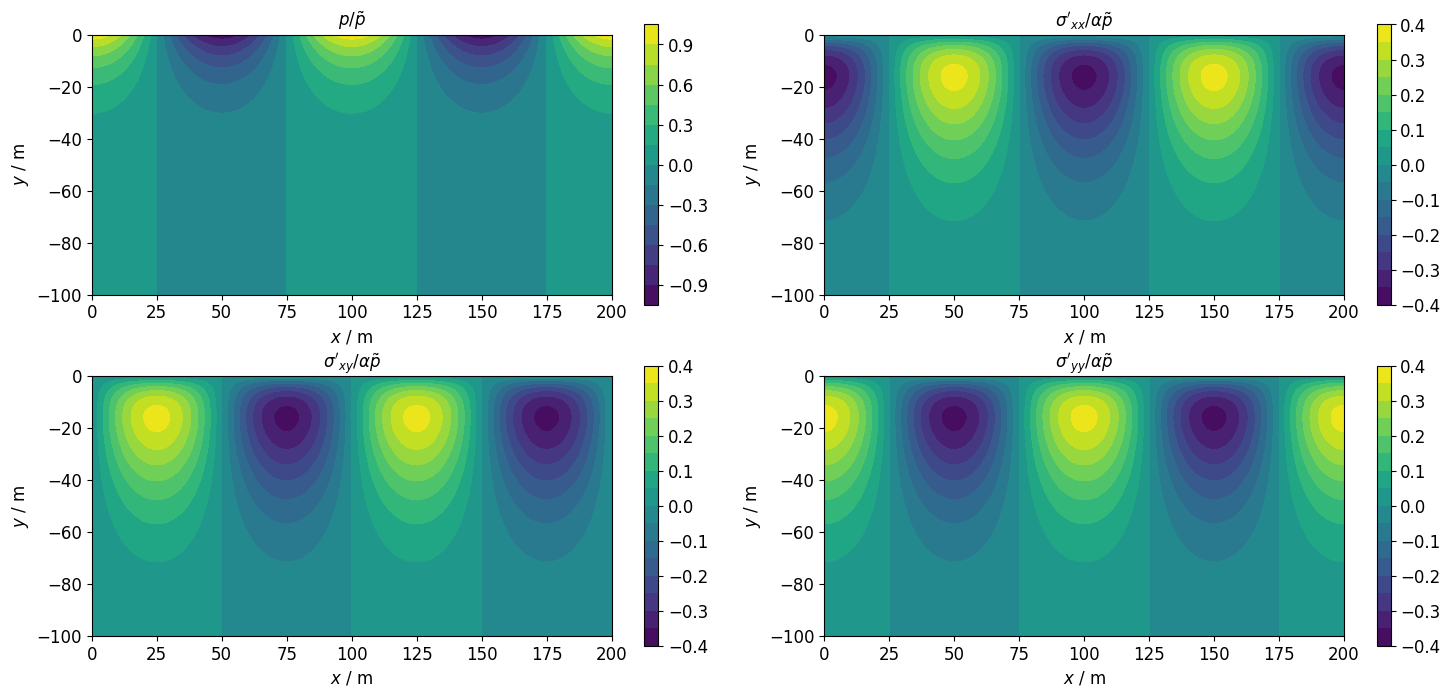
For a better understanding of the planar pressure and stress distribution, the following 2D color-plots are helpful. Each of the diagramms illustrates the pressure or stress distribution at a timepoint, where the applied load is at maximum.
x, y = np.meshgrid(np.linspace(0, 200, 1000), np.linspace(0, 100, 1000))…
(click to toggle)
x, y = np.meshgrid(np.linspace(0, 200, 1000), np.linspace(0, 100, 1000))
t = 2.5

fig, ax = plt.subplots(ncols=2, nrows=2, figsize=(15, 7))
l1 = ax[0][0].contourf(x, -y, compute_pressure_and_stresses(t, x, y)[0], 15)
l2 = ax[0][1].contourf(x, -y, compute_pressure_and_stresses(t, x, y)[1], 15)
l3 = ax[1][1].contourf(x, -y, compute_pressure_and_stresses(t, x, y)[2], 15)
l4 = ax[1][0].contourf(x, -y, compute_pressure_and_stresses(t, x, y)[3], 15)
fig.colorbar(l1, ax=ax[0][0])
fig.colorbar(l2, ax=ax[0][1])
fig.colorbar(l3, ax=ax[1][1])
fig.colorbar(l4, ax=ax[1][0])
for i in (0, 1):
    for j in (0, 1):
        ax[i][j].set_aspect("equal")
        ax[i][j].set_xlabel("$x$ / m")
        ax[i][j].set_ylabel("$y$ / m")
ax[0][0].set_title("$p/\\tilde{p}$")
ax[0][1].set_title("$\\sigma'_{xx}/\\alpha\\tilde{p}$")
ax[1][1].set_title("$\\sigma'_{yy}/\\alpha\\tilde{p}$")
ax[1][0].set_title("$\\sigma'_{xy}/\\alpha\\tilde{p}$")
fig.tight_layout()
Numerical solution
In the following section, the behavior of the seabed under the influence of standing water waves is solved numerically by FEM in OpenGeoSys. The principle of Finite Element Methods is to subdivide a large and complex object into smaller parts (called finite elements), which is achieved by the construction of a mesh of the object. For each of the meshes’ nodes, an approximation of the real solution is calculated. Therefore, numerical solutions always contain errors that originate in the so-called space discretization. The finer the resolution of a mesh, the more accurately the approximation matches the real solution. However, a large number of elements and nodes also causes longer calculation times. A description of the meshing process for this specific example follows below.
For transient problems, a time discretization must also be carried out in addition to the space discretization. In doing so, the observed time period is divided into finite time steps. Here too, smaller timesteps come along with more accurate results but longer calculation times. For the numerical simulation of the seabed, a timestep of $\Delta t = 0.25$ s was chosen. With a periodic time of the water wave of $T=10$ s, there are $40$ timesteps per period. The number of timesteps per period should be large enough to enable an accurate representation of the wave’s sinusoidal shape.
Meshing
Since the problem can be simplified to a planar geometry, a two-dimensional mesh is constructed for the numerical solution. Here, the Gmsh application programming interface (API) for python is used to generate a structured mesh of rectangular shape. This allows a parametric input of the geometry’s dimensions and the mesh refinement. The generated mesh consists of quadratic elements, which have mid-side-nodes. In that way, displacements between nodes at the vertices can be interpolated using a higher order polynomial.
For the further use in OpenGeoSys, the gmsh-mesh is converted to the vtu-format.
out_dir = Path(os.environ.get("OGS_TESTRUNNER_OUT_DIR", "_out"))
out_dir.mkdir(parents=True, exist_ok=True)
def generate_mesh_axb(a, b, Nx, Ny, P):…
(click to toggle)
def generate_mesh_axb(a, b, Nx, Ny, P):
    output_file = f"{out_dir}/square_{a}x{b}.msh"

    lc = 0.5

    # Before using any functions in the Python API, Gmsh must be initialized:
    gmsh.initialize()
    gmsh.option.setNumber("General.Terminal", 1)
    gmsh.model.add("rectangle")

    # Dimensions
    dim1 = 1
    dim2 = 2

    # Outer points (ccw)
    gmsh.model.geo.addPoint(0, -b, 0, lc, 1)
    gmsh.model.geo.addPoint(a, -b, 0, lc, 2)
    gmsh.model.geo.addPoint(a, -b / 2, 0, lc, 3)
    gmsh.model.geo.addPoint(a, 0, 0, lc, 4)
    gmsh.model.geo.addPoint(0, 0, 0, lc, 5)
    gmsh.model.geo.addPoint(0, -b / 2, 0, lc, 6)

    # Outer lines (ccw)
    gmsh.model.geo.addLine(1, 2, 1)
    gmsh.model.geo.addLine(2, 3, 2)
    gmsh.model.geo.addLine(3, 4, 3)
    gmsh.model.geo.addLine(4, 5, 4)
    gmsh.model.geo.addLine(5, 6, 5)
    gmsh.model.geo.addLine(6, 1, 6)
    gmsh.model.geo.addLine(6, 3, 7)

    # The third elementary entity is the surface. In order to define a surface
    # from the curves defined above, a curve loop has first to be defined (ccw).
    gmsh.model.geo.addCurveLoop([1, 2, -7, 6], 1)
    gmsh.model.geo.addCurveLoop([7, 3, 4, 5], 2)

    # Add plane surfaces defined by one or more curve loops.
    gmsh.model.geo.addPlaneSurface([1], 1)
    gmsh.model.geo.addPlaneSurface([2], 2)

    gmsh.model.geo.synchronize()

    #  Prepare structured grid
    gmsh.model.geo.mesh.setTransfiniteCurve(1, Nx)
    gmsh.model.geo.mesh.setTransfiniteCurve(2, int(Ny * 0.3))
    gmsh.model.geo.mesh.setTransfiniteCurve(3, Ny, "Progression", -P)
    gmsh.model.geo.mesh.setTransfiniteCurve(4, Nx)
    gmsh.model.geo.mesh.setTransfiniteCurve(5, Ny, "Progression", P)
    gmsh.model.geo.mesh.setTransfiniteCurve(6, int(Ny * 0.3))
    gmsh.model.geo.mesh.setTransfiniteCurve(7, Nx)

    gmsh.model.geo.mesh.setTransfiniteSurface(1, "Alternate")
    gmsh.model.geo.mesh.setTransfiniteSurface(2, "Alternate")

    gmsh.model.geo.mesh.setRecombine(dim2, 1)
    gmsh.model.geo.mesh.setRecombine(dim2, 2)

    gmsh.model.geo.synchronize()

    # Physical groups (only this gets saved to file per default)
    Bottom = gmsh.model.addPhysicalGroup(dim1, [1])
    gmsh.model.setPhysicalName(dim1, Bottom, "Bottom")

    Right = gmsh.model.addPhysicalGroup(dim1, [2, 3])
    gmsh.model.setPhysicalName(dim1, Right, "Right")

    Top = gmsh.model.addPhysicalGroup(dim1, [4])
    gmsh.model.setPhysicalName(dim1, Top, "Top")

    Left = gmsh.model.addPhysicalGroup(dim1, [5, 6])
    gmsh.model.setPhysicalName(dim1, Left, "Left")

    Plate = gmsh.model.addPhysicalGroup(dim2, [1, 2])
    gmsh.model.setPhysicalName(dim2, Plate, "Plate")

    gmsh.model.geo.synchronize()

    gmsh.model.mesh.generate(dim2)
    # gmsh.option.setNumber('Mesh.SecondOrderIncomplete', 1)   # serendipity elements
    gmsh.model.mesh.setOrder(2)  # higher order elements (quadratic)
    gmsh.write(output_file)

gmsh.finalize()generate_mesh_axb(200, 100, 25, 45, 1.07)Info : Meshing 1D...
Info : [ 0%] Meshing curve 1 (Line)
Info : [ 20%] Meshing curve 2 (Line)
Info : [ 30%] Meshing curve 3 (Line)
Info : [ 50%] Meshing curve 4 (Line)
Info : [ 60%] Meshing curve 5 (Line)
Info : [ 80%] Meshing curve 6 (Line)
Info : [ 90%] Meshing curve 7 (Line)
Info : Done meshing 1D (Wall 0.000716113s, CPU 0.000713s)
Info : Meshing 2D...
Info : [ 0%] Meshing surface 1 (Transfinite)
Info : [ 60%] Meshing surface 2 (Transfinite)
Info : Done meshing 2D (Wall 0.000423331s, CPU 0.000406s)
Info : 1425 nodes 1534 elements
Info : Meshing order 2 (curvilinear on)...
Info : [ 0%] Meshing curve 1 order 2
Info : [ 20%] Meshing curve 2 order 2
Info : [ 30%] Meshing curve 3 order 2
Info : [ 40%] Meshing curve 4 order 2
Info : [ 50%] Meshing curve 5 order 2
Info : [ 60%] Meshing curve 6 order 2
Info : [ 70%] Meshing curve 7 order 2
Info : [ 80%] Meshing surface 1 order 2
Info : [ 90%] Meshing surface 2 order 2
Info : Done meshing order 2 (Wall 0.00508694s, CPU 0.004104s)
Info : Writing '/var/lib/gitlab-runner/builds/t1_R7hwLX/1/ogs/build/release-all/Tests/Data/HydroMechanics/SeabedResponse/Stationary_waves/square_200x100.msh'...
Info : Done writing '/var/lib/gitlab-runner/builds/t1_R7hwLX/1/ogs/build/release-all/Tests/Data/HydroMechanics/SeabedResponse/Stationary_waves/square_200x100.msh'
input_file = f"{out_dir}/square_200x100.msh"…
(click to toggle)
input_file = f"{out_dir}/square_200x100.msh"
meshes = ot.Meshes.from_gmsh(filename=input_file, log=False)
for name, mesh in meshes.items():
pv.save_meshio(f"{out_dir}/square_200x100_{name}.vtu", mesh)info: Reordering nodes...
info: Method: Reversing order of nodes unless it is considered correct by the OGS6 standard, i.e. such that det(J) > 0, where J is the Jacobian of the global-to-local coordinate transformation.
info: Corrected 0 elements.
info: VTU file written.
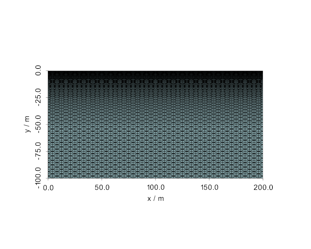
The below figure shows the generated mesh with a width of $a=2L=200$ m and a height (or rather depth) of $b=L=100$ m.
Note: the origin of coordinates is located at ground level, therefore y-coordinates are negative
As was already visible in the analytical solution, the pressure and stress gradients are particularly high in the upper half of the geometry. Therefore, it makes sense to refine the mesh in this area.
pv.set_plot_theme("document")…
(click to toggle)
pv.set_plot_theme("document")
pv.set_jupyter_backend("static")

mesh = pv.read(f"{out_dir}/square_200x100_domain.vtu")
plotter = pv.Plotter(window_size=[1000, 800])
plotter.add_mesh(mesh, show_edges=True, show_scalar_bar=False, color=None, scalars=None)

plotter.show_bounds(ticks="outside", xlabel="x / m", ylabel="y / m")
plotter.view_xy()
plotter.show()[0m[33m2026-05-18 15:52:22.534 ( 5.010s) [ 7FCAFB864400]vtkXOpenGLRenderWindow.:1460 WARN| bad X server connection. DISPLAY=[0m
/tmp/ipykernel_1832228/3628645054.py:8: PyVistaDeprecationWarning: `xlabel` is deprecated. Use `xtitle` instead.
plotter.show_bounds(ticks="outside", xlabel="x / m", ylabel="y / m")
/tmp/ipykernel_1832228/3628645054.py:8: PyVistaDeprecationWarning: `ylabel` is deprecated. Use `ytitle` instead.
plotter.show_bounds(ticks="outside", xlabel="x / m", ylabel="y / m")
Boundary and initial conditions
Because it would not be possible and useful to solve the problem for an infinitely extended seabed, the observed domain has limited dimensions. This however calls for the definition of boundary conditions at the edges of the domain. Boundary conditions constrain the value of a process variable (Dirichlet boundary condition) or the derivative of a process variable applied at the boundary of the domain (Neumann boundary condition). The process variables in this example are the (pore) pressure $p$ and the displacement $u$.
In this example, the boundary conditions are defined as follows:
Top:
$$ \begin{align} p(y=0)&=\tilde{p}\cdot \sin(\omega \cdot t) \cdot \cos(\frac{2 \pi}{L} \cdot x) \\ \sigma_{yy}(y=0)&=-\tilde{p}\cdot \sin(\omega \cdot t) \cdot \cos(\frac{2 \pi}{L} \cdot x) \end{align} $$These boundary conditions represent the applied load in the form of a stationary wave with an amplitude of $\tilde{p} = 0.1\cdot10^5$ Pa. The Neumann boundary condition of the displacement equates to the vertical total stress (Attention: downwards direction is negative).
Bottom:
$$ %\begin{align} u_{y}(y=L) =0 %\end{align} $$Left and right:
$$ \begin{align} u_{x}(x=0)&=0 \\ u_{x}(x=2L)&=0 \end{align} $$Along the vertical lines directly underneath the anti-nodes of the wave, there is no horizontal displacement. Since the maximum loads appear in that area, the material evades symmetrically to both sides from this line to places of lower stress. For this reason, the vertical boundaries of the domain are chosen exactly along these lines.
Since the problem is time-dependent, initial conditions must be specified as well:
$$ \begin{align} \vec{u}(t=0)&=\vec{0} \\ p(t=0)&=0 \textsf{ Pa} \end{align} $$Running the numerical model
## Helper Functions…
(click to toggle)
## Helper Functions
def read_timestep_mesh(a, time):
    reader = pv.PVDReader(f"{out_dir}/square_{a}x100.pvd")
    reader.set_active_time_point(int(time * 4))  # time [s], delta t = 0.25 s
    return reader.read()[0]


def slice_along_line(mesh, start_point, end_point):
    line = pv.Line(start_point, end_point, resolution=2)
    return mesh.slice_along_line(line)


def get_pressure_sorted(mesh):
    pressure = mesh.point_data["pressure_interpolated"]
    depth = mesh.points[:, 1]
    indices_sorted = np.argsort(depth)
    return pressure[indices_sorted]


def get_stresses_sorted(mesh):
    sigma = mesh.point_data["sigma"]
    depth = mesh.points[:, 1]
    indices_sorted = np.argsort(depth)
    sigma_xx = -sigma[indices_sorted, 0]  # switching sign convention
    sigma_yy = -sigma[indices_sorted, 1]
    # sigma_zz = - sigma[indices_sorted, 2]
    sigma_xy = +sigma[indices_sorted, 3]
    return sigma_xx, sigma_yy, sigma_xy  # ,sigma_zz


def get_depth_sorted(mesh):
    depth = mesh.points[:, 1]
    indices_sorted = np.argsort(depth)
    return depth[indices_sorted]


def compute_abs_and_rel_pressure_error(pressures, depth, t, x):
    num_points = pressures.shape[0]
    f_abs = np.zeros(num_points)
    f_rel = np.zeros(num_points)

    for pt_idx in range(num_points):
        y = -depth[pt_idx]
        pressure_ana = compute_pressure_and_stresses(t, x, y)[
            0
        ]  # returns pressure normalised to the pressure amplitude
        pressure_num = (
            pressures[pt_idx] / 0.1e5
        )  # absolute pressure divided by pressure amplitude
        f_abs[pt_idx] = pressure_num - pressure_ana

        if pressure_ana == 0:
            f_rel[pt_idx] = f_abs[pt_idx] / 1e-2
        else:
            f_rel[pt_idx] = f_abs[pt_idx] / pressure_ana

    return f_abs, f_rel


def compute_abs_and_rel_stress_error(_sigmas, depth, t, x):
    num_points = depth.shape[0]
    f_abs = np.zeros((3, num_points))
    f_rel = np.zeros((3, num_points))

    for stress_idx in (0, 1, 2):
        for pt_idx in range(num_points):
            y = -depth[pt_idx]
            sigma_ana = compute_pressure_and_stresses(t, x, y)[
                stress_idx + 1
            ]  # returns stresses normalised to the pressure amplitude
            sigma_num = (
                sigma[stress_idx][pt_idx] / 0.1e5
            )  # absolute stresses divided by pressure amplitude
            f_abs[stress_idx][pt_idx] = sigma_num - sigma_ana

            if sigma_ana == 0:
                f_rel[stress_idx][pt_idx] = f_abs[stress_idx][pt_idx] / 1e-2
            else:
                f_rel[stress_idx][pt_idx] = f_abs[stress_idx][pt_idx] / sigma_ana

    return f_abs, f_rel
model = ot.Project(…
(click to toggle)
model = ot.Project(
    input_file="seabed_response_200x100.prj",
    output_file=out_dir / "seabed_response_200x100.prj",
)
model.write_input()
model.run_model(logfile=f"{out_dir}/out.txt", args=f"-o {out_dir} -m {out_dir}") ogs -o /var/lib/gitlab-runner/builds/t1_R7hwLX/1/ogs/build/release-all/Tests/Data/HydroMechanics/SeabedResponse/Stationary_waves -m /var/lib/gitlab-runner/builds/t1_R7hwLX/1/ogs/build/release-all/Tests/Data/HydroMechanics/SeabedResponse/Stationary_waves /var/lib/gitlab-runner/builds/t1_R7hwLX/1/ogs/build/release-all/Tests/Data/HydroMechanics/SeabedResponse/Stationary_waves/seabed_response_200x100.prj
['ogs', '-o', '/var/lib/gitlab-runner/builds/t1_R7hwLX/1/ogs/build/release-all/Tests/Data/HydroMechanics/SeabedResponse/Stationary_waves', '-m', '/var/lib/gitlab-runner/builds/t1_R7hwLX/1/ogs/build/release-all/Tests/Data/HydroMechanics/SeabedResponse/Stationary_waves', '/var/lib/gitlab-runner/builds/t1_R7hwLX/1/ogs/build/release-all/Tests/Data/HydroMechanics/SeabedResponse/Stationary_waves/seabed_response_200x100.prj']
<Popen: returncode: 0 args: ' ogs -o /var/lib/gitlab-runner/builds/t1_R7hwLX...>
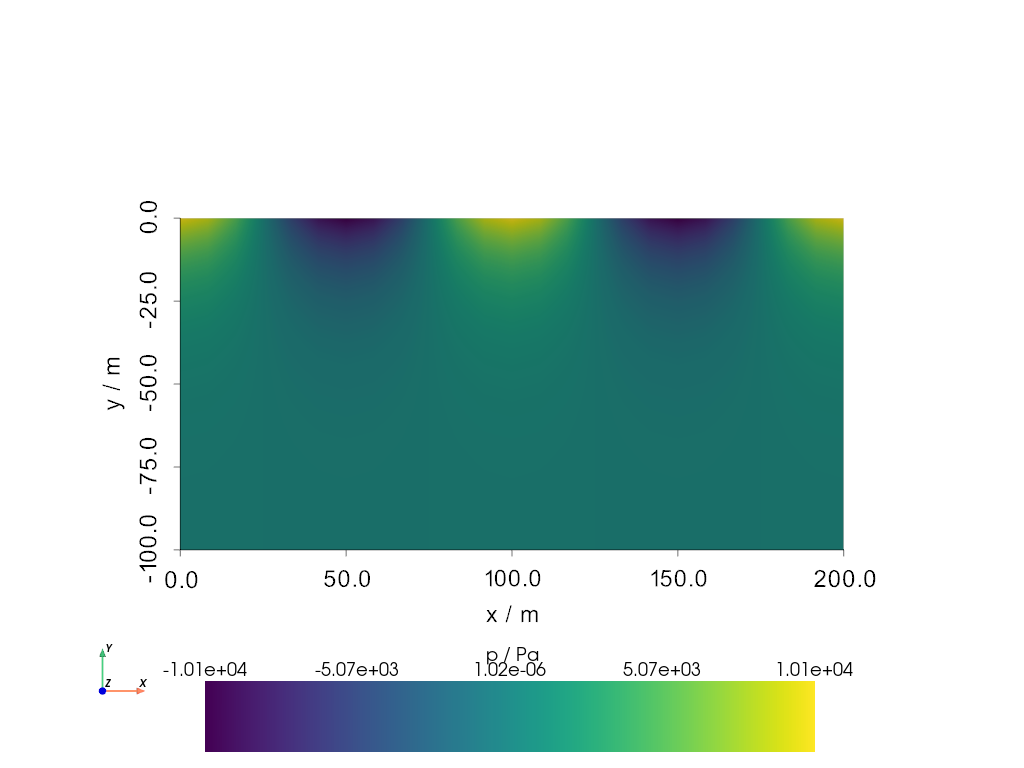
The below plot illustrates the pore pressure distribution in the domain at a timepoint where the applied load is at maximum. By comparing this plot to the 2D-colorplots of the analytical solution, it can already be concluded that the numerical solution resembles the analytical solution.
time = 2.5 # [s]…
(click to toggle)
time = 2.5  # [s]
reader = pv.get_reader(f"{out_dir}/square_200x100.pvd")
reader.set_active_time_point(int(time * 4))
mesh = reader.read()[0]

plotter = pv.Plotter()

sargs = dict(title="p / Pa", height=0.25, position_x=0.2, position_y=0.02)  # noqa: C408
plotter.add_mesh(
    mesh,
    scalars="pressure_interpolated",
    show_edges=False,
    show_scalar_bar=True,
    label="p",
    scalar_bar_args=sargs,
)
plotter.show_bounds(ticks="outside", xlabel="x / m", ylabel="y / m")
plotter.add_axes()
plotter.view_xy()
plotter.show()/tmp/ipykernel_1832228/731124242.py:17: PyVistaDeprecationWarning: `xlabel` is deprecated. Use `xtitle` instead.
plotter.show_bounds(ticks="outside", xlabel="x / m", ylabel="y / m")
/tmp/ipykernel_1832228/731124242.py:17: PyVistaDeprecationWarning: `ylabel` is deprecated. Use `ytitle` instead.
plotter.show_bounds(ticks="outside", xlabel="x / m", ylabel="y / m")
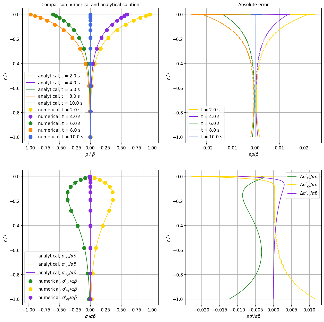
For a more detailed comparison between the analytical and the numerical solution, both solutions are evaluated along the vertical line directly underneath an anti-node of the standing wave. As before, the pore pressure and the amplitude of the effective stresses are illustrated as a function of depth. The results of the numerical solution are marked as dots in the same color as the analytical solution. Additionally, the absolute errors $\Delta p = p_{numerical}-p_{analtical}$ and $\Delta \sigma_{i}' = \sigma_{i, numerical}'-\sigma_{i, analytical}'$ are illustrated on the right.
The plot shows that the absolute errors are very small at about $2 \%$ of the wave’s amplitude. They can mostly be ascribed to the space- and time-discretization. Close to the top boundary of the domain, larger errors occur. These errors could originate in the definition of both a pressure and displacement (Neumann-) boundary condition along the top edge.
x = 0…
(click to toggle)
x = 0
y = np.linspace(0, 100, 1000)
y_rel = y / 100
colors = {
    0: "orangered",
    2: "gold",
    4: "blueviolet",
    6: "forestgreen",
    8: "darkorange",
    10: "royalblue",
}

fig, ax = plt.subplots(ncols=2, nrows=2, figsize=(15, 15))

## Plotting analytical solution
for t in [2, 4, 6, 8, 10]:
    ax[0][0].plot(
        compute_pressure_and_stresses(t, x, y)[0],
        -y_rel,
        color=colors[t],
        label=f"analytical, t = {t:.1f} s",
    )

ax[1][0].plot(
    compute_pressure_and_stresses(2.5, x, y)[1],
    -y_rel,
    color=colors[6],
    label="analytical, $\\sigma'_{xx}/\\alpha\\tilde{p}$",
)
ax[1][0].plot(
    compute_pressure_and_stresses(2.5, x, y)[2],
    -y_rel,
    color=colors[2],
    label="analytical, $\\sigma'_{yy}/\\alpha\\tilde{p}$",
)
ax[1][0].plot(
    compute_pressure_and_stresses(2.5, x, y)[3],
    -y_rel,
    color=colors[4],
    label="analytical, $\\sigma'_{xy}/\\alpha\\tilde{p}$",
)

## Plotting numerical solution
p1 = (x + 1e-6, 0, 0)
p2 = (x + 1e-6, -100, 0)

for t_num in (2, 2.5, 4, 6, 8, 10):
    mesh = read_timestep_mesh(200, t_num)

    line_mesh = slice_along_line(mesh, p1, p2)
    pressure = get_pressure_sorted(line_mesh)
    sigma = get_stresses_sorted(line_mesh)
    depth = get_depth_sorted(line_mesh)
    f_abs_pressure = compute_abs_and_rel_pressure_error(pressure, depth, t_num, x)[0]
    f_abs_sigma = compute_abs_and_rel_stress_error(sigma, depth, t_num, x)[0]

    if t_num != 2.5:
        ax[0][0].plot(
            pressure / 0.1e5,
            depth / 100,
            "o",
            markevery=10,
            color=colors[t_num],
            label=f"numerical, t = {t_num:.1f} s",
        )
        ax[0][0].set_xlabel("$p$ / $\\tilde{p}$")

        ax[0][1].plot(
            f_abs_pressure, depth / 100, color=colors[t_num], label=f"t = {t_num:.1f} s"
        )
        ax[0][1].set_xlabel("$\\Delta p /\\tilde{p}$")

    if t_num == 2.5:
        ax[1][0].plot(
            sigma[0] / 0.1e5,
            depth / 100,
            "o",
            markevery=10,
            color=colors[6],
            label="numerical, $\\sigma'_{xx}/\\alpha\\tilde{p}$",
        )
        ax[1][0].plot(
            sigma[1] / 0.1e5,
            depth / 100,
            "o",
            markevery=10,
            color=colors[2],
            label="numerical, $\\sigma'_{yy}/\\alpha\\tilde{p}$",
        )
        ax[1][0].plot(
            sigma[2] / 0.1e5,
            depth / 100,
            "o",
            markevery=10,
            color=colors[4],
            label="numerical, $\\sigma'_{xy}/\\alpha\\tilde{p}$",
        )
        ax[1][0].set_xlabel("$\\sigma$'/$\\alpha\\tilde{p}$")

        ax[1][1].plot(
            f_abs_sigma[0],
            depth / 100,
            color=colors[6],
            label="$\\Delta\\sigma'_{xx}/\\alpha\\tilde{p}$",
        )
        ax[1][1].plot(
            f_abs_sigma[1],
            depth / 100,
            color=colors[2],
            label="$\\Delta\\sigma'_{yy}/\\alpha\\tilde{p}$",
        )
        ax[1][1].plot(
            f_abs_sigma[2],
            depth / 100,
            color=colors[4],
            label="$\\Delta\\sigma'_{xy}/\\alpha\\tilde{p}$",
        )
        ax[1][1].set_xlabel("$\\Delta\\sigma$'/$\\alpha\\tilde{p}$")

        # ax[1][0].plot(sigma[3]/0.1e5, depth/100, "o", markevery=10, color = colors[4], label = "numerical, $\\sigma'_{zz}/\\alpha\\tilde{p}$")

## layout settings
ax[0][0].set_title("Comparison numerical and analytical solution")
ax[0][1].set_title("Absolute error")

for idx_1 in (0, 1):
    for idx_2 in (0, 1):
        ax[idx_1][idx_2].grid(True)
        ax[idx_1][idx_2].set_ylabel("$y$ / $L$")
        ax[idx_1][0].set_xlim(-1.1, 1.1)
        ax[idx_1][idx_2].legend()
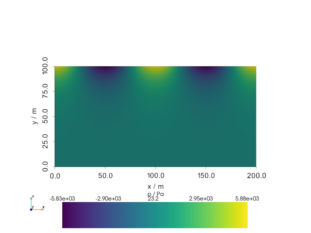
FEniCSx
The FEniCSx script used for the numerical simulation is based on the hydro-mechanical model described in [4] and provided as the attached Python script (Seabed_response_fenicsx.py). The model is applicable for finite deformations due to the chosen kinematic approach and is formulated within a total Lagrangian framework. In contrast to [4], a simplified permeability approach was chosen, while still a compressible fluid and the same stress-strain approach were used (hyperelastic compressible Neo-Hookean approach), but without a tension cut-off. Apart from that, the simulations in [4] were performed using FEniCS (version 2019.2.0.13.dev0), whereas this benchmark uses FEniCSx (version 0.10.0).
with (out_dir / "seabed_response_dolfinx.log").open("w") as log_file:…
(click to toggle)
with (out_dir / "seabed_response_dolfinx.log").open("w") as log_file:
    subprocess.run(
        [
            "docker",
            "run",
            "-i",
            "--rm",
            "--entrypoint",
            "/dolfinx-env/bin/python",
            "-v",
            f"{Path.cwd()}:/root/shared",
            "-v",
            f"{out_dir}:/root/results",
            "-w",
            "/root/shared",
            "dolfinx/dolfinx:v0.10.0",
            "seabed_response_dolfinx.py",
            "--result-folder",
            "/root/results",
        ],
        check=True,
        stdout=log_file,
        stderr=subprocess.STDOUT,
)Post-processing
def xdmf_to_vtu(xdmf_path, step):…
(click to toggle)
def xdmf_to_vtu(xdmf_path, step):
    with meshio.xdmf.TimeSeriesReader(xdmf_path + ".xdmf") as reader:

        points, cells = reader.read_points_cells()

        if points.shape[1] == 2:
            points = np.column_stack([points, np.zeros(points.shape[0])])

        for k in range(0, reader.num_steps, step):

            t, point_data, cell_data = reader.read_data(k)

            mesh = meshio.Mesh(
                points=points, cells=cells, point_data=point_data, cell_data=cell_data
            )

            outname = f"{xdmf_path}_step_{k:04d}_t_{t:.3f}.vtu"
meshio.write(outname, mesh)xdmf_to_vtu(str(out_dir / "seabed_constant_p"), 20)
xdmf_to_vtu(str(out_dir / "seabed_constant_stress"), 20)
reader = pv.get_reader(str(out_dir / "seabed_constant_p_step_0000_t_0.000.vtu"))…
(click to toggle)
reader = pv.get_reader(str(out_dir / "seabed_constant_p_step_0000_t_0.000.vtu"))
mesh_t0 = reader.read()

reader = pv.get_reader(str(out_dir / "seabed_constant_p_step_0020_t_2.000.vtu"))
mesh_t2 = reader.read()

reader = pv.get_reader(str(out_dir / "seabed_constant_p_step_0040_t_4.000.vtu"))
mesh_t4 = reader.read()

reader = pv.get_reader(str(out_dir / "seabed_constant_p_step_0060_t_6.000.vtu"))
mesh_t6 = reader.read()

reader = pv.get_reader(str(out_dir / "seabed_constant_p_step_0080_t_8.000.vtu"))
mesh_t8 = reader.read()

reader = pv.get_reader(str(out_dir / "seabed_constant_p_step_0100_t_10.000.vtu"))
mesh_t10 = reader.read()
plotter = pv.Plotter()…
(click to toggle)
plotter = pv.Plotter()
sargs = dict(title="p / Pa", height=0.3, position_x=0.2, position_y=0.02)  # noqa: C408
plotter.add_mesh(
    mesh_t4,
    scalars="Porewater pressure",
    show_edges=False,
    show_scalar_bar=True,
    label="p",
    scalar_bar_args=sargs,
)
plotter.show_bounds(ticks="outside", xtitle="x / m", ytitle="y / m")
plotter.add_axes()
plotter.view_xy()
plotter.show()
reader = pv.get_reader(str(out_dir / "seabed_constant_stress_step_0000_t_0.000.vtu"))…
(click to toggle)
reader = pv.get_reader(str(out_dir / "seabed_constant_stress_step_0000_t_0.000.vtu"))
mesh_t0_stress = reader.read()

reader = pv.get_reader(str(out_dir / "seabed_constant_stress_step_0020_t_2.000.vtu"))
mesh_t2_stress = reader.read()

reader = pv.get_reader(str(out_dir / "seabed_constant_stress_step_0040_t_4.000.vtu"))
mesh_t4_stress = reader.read()

reader = pv.get_reader(str(out_dir / "seabed_constant_stress_step_0060_t_6.000.vtu"))
mesh_t6_stress = reader.read()

reader = pv.get_reader(str(out_dir / "seabed_constant_stress_step_0080_t_8.000.vtu"))
mesh_t8_stress = reader.read()

reader = pv.get_reader(str(out_dir / "seabed_constant_stress_step_0100_t_10.000.vtu"))
mesh_t10_stress = reader.read()
def nodes_along_line_FEniCSx(mesh):…
(click to toggle)
def nodes_along_line_FEniCSx(mesh):
    tolerance = 1e-8
    mask = np.abs(mesh.points[:, 0]) < tolerance  # boolean whether node lays at x=0
    line_points = mesh.points[mask]
    order = np.argsort(line_points[:, 1])
    line_points = line_points[order]  # node points along x=0

    return mask, line_points


def get_pressure_sorted_FEniCSx(mesh, mask, line_points):
    pressure = mesh.point_data["Porewater pressure"][mask]
    depth = line_points[:, 1]
    indices_sorted = np.argsort(depth)
    return pressure[indices_sorted]


def get_depth_sorted_nodes_FEniCSx(line_points):
    depth = line_points[:, 1]
    indices_sorted = np.argsort(depth)
    return depth[indices_sorted]


def get_stresses_sorted_FEniCSx(mesh, mask, line_points):
    sigma = mesh.point_data["Cauchy"][mask]
    depth = line_points[:, 1]
    indices_sorted = np.argsort(depth)
    sigma_xx = -sigma[indices_sorted, 0]
    sigma_yy = -sigma[indices_sorted, 3]
    sigma_xy = -sigma[indices_sorted, 1]
    return sigma_xx, sigma_yy, sigma_xy
def compute_abs_and_rel_pressure_error_FEniCSx(pressures, depth, t, x):…
(click to toggle)
def compute_abs_and_rel_pressure_error_FEniCSx(pressures, depth, t, x):
    num_points = pressures.shape[0]
    f_abs = np.zeros(num_points)

    analytical_index = np.arange(num_points)
    numerical_index = np.arange(num_points - 1, -1, -1)

    for ana_idx, num_idx in zip(analytical_index, numerical_index, strict=False):
        y = depth[ana_idx]
        pressure_ana = compute_pressure_and_stresses(t, x, y)[
            0
        ]  # returns pressure normalised to the pressure amplitude #calculated from top to bottom
        pressure_num = (
            pressures[num_idx] / 0.1e5
        )  # absolute pressure divided by pressure amplitude       #calculated originally from bottom to top - num idx guarantees that parameters from top to bottom are called

        f_abs[num_idx] = (
            pressure_num - pressure_ana
        )  # saving with num_idx guarantees a saving from bottom to top (later it is plotted from bottom to top)

    return f_abs


def compute_abs_and_rel_stress_error_FEniCSx(sigma_yy, sigma_xx, sigma_xy, depth, t, x):
    num_points = depth.shape[0]
    f_abs_sigma_yy = np.zeros(num_points)
    f_abs_sigma_xx = np.zeros(num_points)
    f_abs_sigma_xy = np.zeros(num_points)
    analytical_index = np.arange(num_points)
    numerical_index = np.arange(num_points - 1, -1, -1)

    for ana_idx, num_idx in zip(analytical_index, numerical_index, strict=False):
        y = depth[ana_idx]
        sigma_ana_yy = compute_pressure_and_stresses(t, x, y)[
            2
        ]  # returns stresses normalised to the pressure amplitude #calculated from top to bottom
        sigma_ana_xx = compute_pressure_and_stresses(t, x, y)[
            1
        ]  # returns stresses normalised to the pressure amplitude
        sigma_ana_xy = compute_pressure_and_stresses(t, x, y)[3]

        sigma_num_yy = (
            sigma_yy[num_idx] / 0.1e5
        )  # absolute stresses divided by pressure amplitude     #calculated originally from bottom to top - num idx guarantees that parameters from top to bottom are called
        sigma_num_xx = sigma_xx[num_idx] / 0.1e5
        sigma_num_xy = sigma_xy[num_idx] / 0.1e5

        f_abs_sigma_yy[num_idx] = (
            sigma_num_yy - sigma_ana_yy
        )  # saving with num_idx guarantees a saving from bottom to top (later it is plotted from bottom to top)
        f_abs_sigma_xx[num_idx] = sigma_num_xx - sigma_ana_xx
        f_abs_sigma_xy[num_idx] = sigma_num_xy - sigma_ana_xy

    return f_abs_sigma_yy, f_abs_sigma_xx, f_abs_sigma_xy
x = 0…
(click to toggle)
x = 0
y = np.linspace(0, 100, 1000)
y_rel = y / 100

fig, ax = plt.subplots(ncols=2, nrows=2, figsize=(15, 15))

## Plotting analytical solution
for t in [2, 4, 6, 8, 10]:
    if t != 10:
        ax[0][0].plot(
            compute_pressure_and_stresses(t, x, y)[0],
            -y_rel,
            color=colors[t],
            alpha=0.6,
        )
    else:
        (ANALYTICAL,) = ax[0][0].plot(
            compute_pressure_and_stresses(t, x, y)[0],
            -y_rel,
            color=colors[t],
            alpha=0.6,
            label="analytical",
        )

ax[1][0].plot(
    compute_pressure_and_stresses(2, x, y)[1],
    -y_rel,
    color=colors[6],
    label="analytical, $\\sigma'_{xx}$ / $\\alpha\\tilde{p}$",
)
ax[1][0].plot(
    compute_pressure_and_stresses(2, x, y)[2],
    -y_rel,
    color=colors[2],
    label="analytical, $\\sigma'_{yy}$ / $\\alpha\\tilde{p}$",
)
ax[1][0].plot(
    compute_pressure_and_stresses(2, x, y)[3],
    -y_rel,
    color=colors[4],
    label="analytical, $\\sigma'_{xy}$ / $\\alpha\\tilde{p}$",
)

i_steps = [2, 4, 6, 8, 10]
meshes = [mesh_t2, mesh_t4, mesh_t6, mesh_t8, mesh_t10]
meshes_stress = [mesh_t2_stress]

for step, mesh in zip(i_steps, meshes, strict=False):
    mask, line_points = nodes_along_line_FEniCSx(mesh)
    pressure = get_pressure_sorted_FEniCSx(mesh, mask, line_points)
    depth = get_depth_sorted_nodes_FEniCSx(line_points)
    f_abs_pressure = compute_abs_and_rel_pressure_error_FEniCSx(
        pressure, depth, step, x
    )

    if step != 10:
        ax[0][0].plot(pressure / 0.1e5, (depth / 100) - 1, "o", color=colors[step])
    else:
        ax[0][0].plot(
            pressure / 0.1e5,
            (depth / 100) - 1,
            "o",
            color=colors[step],
            label="numerical - FEniCSx",
        )

    ax[0][0].set_xlabel("$p$ / $\\tilde{p}$")
    ax[0][0].set_ylabel("$y$ / L")
    ax[0][0].set_xlim(-1.1, 1.1)
    ax[0][0].grid(True)

    ax[0][1].plot(
        f_abs_pressure,
        (depth / 100) - 1,
        "o",
        color=colors[step],
        label=f"t = {step:.1f} s",
    )
    ax[0][1].set_xlabel("$\\Delta p$ / $\\tilde{p}$")
    ax[0][1].grid(True)
    ax[0][0].set_ylabel("$y$ / L")

# Add the first legend
first_patch = mpatches.Patch(color=colors[2], label="$t = 2.0$ s")
second_patch = mpatches.Patch(color=colors[4], label="$t = 4.0$ s")
third_patch = mpatches.Patch(color=colors[6], label="$t = 6.0$ s")
forth_patch = mpatches.Patch(color=colors[8], label="$t = 8.0$ s")
fifth_patch = mpatches.Patch(color=colors[10], label="$t = 10.0$ s")

first_legend = ax[0][0].legend(
    handles=[first_patch, second_patch, third_patch, forth_patch, fifth_patch],
    loc="lower left",
)

# Manually add the first legend back to the plot
ax[0][0].add_artist(first_legend)
ax[0][0].legend(bbox_to_anchor=(0.52, 0.15))

for step, mesh_stress in zip(i_steps, meshes_stress, strict=False):

    mask, line_points = nodes_along_line_FEniCSx(mesh_stress)
    sigma_xx, sigma_yy, sigma_xy = get_stresses_sorted_FEniCSx(
        mesh_stress, mask, line_points
    )
    depth = get_depth_sorted_nodes_FEniCSx(line_points)

    f_abs_sigma_yy, f_abs_sigma_xx, f_abs_sigma_xy = (
        compute_abs_and_rel_stress_error_FEniCSx(
            sigma_yy, sigma_xx, sigma_xy, depth, step, x
        )
    )

    if step == 2:
        ax[1][0].plot(
            sigma_xx / 0.1e5,
            (depth / 100) - 1,
            "o",
            color=colors[6],
            label="numerical, $\\sigma'_{xx}$ / $\\alpha\\tilde{p}$",
        )
        ax[1][0].plot(
            sigma_yy / 0.1e5,
            (depth / 100) - 1,
            "o",
            color=colors[2],
            label="numercal, $\\sigma'_{yy}$ / $\\alpha\\tilde{p}$",
        )
        ax[1][0].plot(
            sigma_xy / 0.1e5,
            (depth / 100) - 1,
            "o",
            color=colors[4],
            label="numerical, $\\sigma'_{xy}$ / $\\alpha\\tilde{p}$",
        )
        ax[1][0].set_xlabel("$\\sigma$' / $\\alpha\\tilde{p}$")
        ax[1][0].set_ylabel("$y$ / L")
        ax[1][0].set_xlim(-1.1, 1.1)
        ax[1][0].grid(True)
        ax[1][0].text(
            0.8,
            0.05,
            "$t = 2.0$ s",
            transform=ax[1][0].transAxes,
            bbox={
                "facecolor": "white",
                "edgecolor": "black",
                "boxstyle": "round,pad=0.5",
                "alpha": 0.9,
            },
        )
        ax[1][0].legend()

        ax[1][1].plot(
            f_abs_sigma_yy,
            (depth / 100) - 1,
            "o",
            color=colors[2],
            label="$\\Delta\\sigma'_{yy}$ / $\\alpha\\tilde{p}$",
        )
        ax[1][1].plot(
            f_abs_sigma_xx,
            (depth / 100) - 1,
            "o",
            color=colors[6],
            label="$\\Delta\\sigma'_{xx}$ / $\\alpha\\tilde{p}$",
        )
        ax[1][1].plot(
            f_abs_sigma_xy,
            (depth / 100) - 1,
            "o",
            color=colors[4],
            label="$\\Delta\\sigma'_{xy}$ / $\\alpha\\tilde{p}$",
        )
        ax[1][1].set_xlabel("$\\Delta\\sigma'$ / $\\alpha\\tilde{p}$")
        ax[1][1].grid(True)

plt.savefig(str(out_dir / "comparison_analytical_fenicsx_p_sigma_error.pdf"))
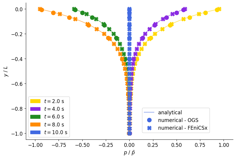
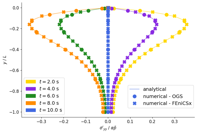
Comparison between FEniCSx, OpenGeoSys and the analytical solution
In the field of numerical simulations, it is good practice to perform Verification and Validation (V&V) in order to build confidence in the results [5]. Verification can be done by comparing results with analytical solutions or with other independent code implementations (see [6] for an example of Quality assurance (QA) of TH²M simulations). The more complex a model is, the more equations and physical components it contains. When using hierarchical benchmarking, the complexity can be increased slowly in order to examine different aspects and simplifications [7].
The following compares the results of the numerical simulation using OpenGeoSys with those of the FEniCSx simulation and the analytical solution.
x = 0…
(click to toggle)
x = 0
y = np.linspace(0, 100, 1000)
y_rel = y / 100

fig, ax = plt.subplots(figsize=(9, 6))
ax.spines["right"].set_color(
    "none"
)  # https://www.grund-wissen.de/informatik/python/scipy/matplotlib.html
ax.spines["top"].set_color(
    "none"
)  # https://www.grund-wissen.de/informatik/python/scipy/matplotlib.html

## Plotting analytical solution
for t in [2, 4, 6, 8, 10]:
    if t != 10:
        ax.plot(
            compute_pressure_and_stresses(t, x, y)[0],
            -y_rel,
            color=colors[t],
            alpha=0.6,
        )
    else:
        (ANALYTICAL,) = ax.plot(
            compute_pressure_and_stresses(t, x, y)[0],
            -y_rel,
            color=colors[t],
            alpha=0.6,
            label="analytical",
        )

## Plotting numerical solution OGS
p1 = (x + 1e-6, 0, 0)
p2 = (x + 1e-6, -100, 0)

for t_num in (2, 4, 6, 8, 10):
    mesh_ogs = read_timestep_mesh(200, t_num)

    line_mesh_ogs = slice_along_line(mesh_ogs, p1, p2)
    pressure_ogs = get_pressure_sorted(line_mesh_ogs)
    depth_ogs = get_depth_sorted(line_mesh_ogs)

    if t_num != 10:
        ax.plot(
            pressure_ogs / 0.1e5,
            depth_ogs / 100,
            "o",
            markevery=15,
            color=colors[t_num],
        )
        ax.set_xlabel("$p$ / $\\tilde{p}$")

    else:
        (OGS,) = ax.plot(
            pressure_ogs / 0.1e5,
            depth_ogs / 100,
            "o",
            markevery=15,
            color=colors[t_num],
            label="numerical - OGS",
        )
        ax.set_xlabel("$p$ / $\\tilde{p}$")

## Plotting numerical solution FEniCSx
i_steps = [2, 4, 6, 8, 10]
meshes = [mesh_t2, mesh_t4, mesh_t6, mesh_t8, mesh_t10]

for step, mesh in zip(i_steps, meshes, strict=False):
    mask, line_points = nodes_along_line_FEniCSx(mesh)
    pressure = get_pressure_sorted_FEniCSx(mesh, mask, line_points)
    depth = get_depth_sorted_nodes_FEniCSx(line_points)
    if step != 10:
        ax.plot(pressure / 0.1e5, (depth / 100) - 1, "X", color=colors[step])
        ax.set_xlabel("$p$ / $\\tilde{p}$")
    else:
        ax.plot(
            pressure / 0.1e5,
            (depth / 100) - 1,
            "X",
            color=colors[step],
            label="numerical - FEniCSx",
        )
        ax.set_xlabel("$p$ / $\\tilde{p}$")

# Add the first legend
first_patch = mpatches.Patch(color=colors[2], label="$t = 2.0$ s")
second_patch = mpatches.Patch(color=colors[4], label="$t = 4.0$ s")
third_patch = mpatches.Patch(color=colors[6], label="$t = 6.0$ s")
forth_patch = mpatches.Patch(color=colors[8], label="$t = 8.0$ s")
fifth_patch = mpatches.Patch(color=colors[10], label="$t = 10.0$ s")

first_legend = ax.legend(
    handles=[first_patch, second_patch, third_patch, forth_patch, fifth_patch],
    loc="lower left",
)

# Manually add the first legend back to the plot
ax.add_artist(first_legend)
ax.legend(bbox_to_anchor=(0.55, 0.25))

# ax.grid(True)
ax.set_ylabel("$y$ / $L$")
ax.set_xlim(-1.1, 1.1)
# ax.legend(bbox_to_anchor=(.55, 0.4))
plt.savefig(str(out_dir / "./comparison_analytical_ogs_fenicsx_p.pdf"))
x = 0…
(click to toggle)
x = 0
y = np.linspace(0, 100, 1000)
y_rel = y / 100

fig, ax = plt.subplots(figsize=(9, 6))
ax.spines["right"].set_color(
    "none"
)  # https://www.grund-wissen.de/informatik/python/scipy/matplotlib.html
ax.spines["top"].set_color(
    "none"
)  # https://www.grund-wissen.de/informatik/python/scipy/matplotlib.html

## Plotting analytical solution
for t in [2, 4, 6, 8, 10]:
    if t != 10:
        ax.plot(
            compute_pressure_and_stresses(t, x, y)[2],
            -y_rel,
            color=colors[t],
            alpha=0.6,
        )
    else:
        (ANALYTICAL,) = ax.plot(
            compute_pressure_and_stresses(t, x, y)[2],
            -y_rel,
            color=colors[t],
            alpha=0.6,
            label="analytical",
        )

## Plotting numerical solution OGS
p1 = (x + 1e-6, 0, 0)
p2 = (x + 1e-6, -100, 0)

for t_num in (2, 4, 6, 8, 10):
    mesh_ogs = read_timestep_mesh(200, t_num)
    line_mesh_ogs = slice_along_line(mesh_ogs, p1, p2)
    pressure_ogs = get_pressure_sorted(line_mesh_ogs)
    sigma_ogs = get_stresses_sorted(line_mesh_ogs)
    depth_ogs = get_depth_sorted(line_mesh_ogs)

    if t_num != 10:
        ax.plot(
            sigma_ogs[1] / 0.1e5,
            depth_ogs / 100,
            "o",
            markevery=15,
            color=colors[t_num],
        )
        ax.set_xlabel("$\\sigma'_{yy,\\text{ogs}}/\\alpha\\tilde{p}$")

    else:
        (OGS,) = ax.plot(
            sigma_ogs[1] / 0.1e5,
            depth_ogs / 100,
            "o",
            markevery=15,
            color=colors[t_num],
            label="numerical - OGS",
        )
        ax.set_xlabel("$\\sigma'_{yy,\\text{ogs}}/\\alpha\\tilde{p}$")

## Plotting numerical solution FEniCSx
i_steps = [2, 4, 6, 8, 10]
meshes_stress = [
    mesh_t2_stress,
    mesh_t4_stress,
    mesh_t6_stress,
    mesh_t8_stress,
    mesh_t10_stress,
]

for step, mesh in zip(i_steps, meshes_stress, strict=False):
    mask, line_points = nodes_along_line_FEniCSx(mesh)
    sigma_xx, sigma_yy, sigma_xy = get_stresses_sorted_FEniCSx(mesh, mask, line_points)
    depth = get_depth_sorted_nodes_FEniCSx(line_points)

    if step != 10:
        ax.plot(sigma_yy / 0.1e5, (depth / 100) - 1, "X", color=colors[step])
        ax.set_xlabel("$\\sigma'_{yy}$ / $\\alpha\\tilde{p}$")
    else:
        ax.plot(
            sigma_yy / 0.1e5,
            (depth / 100) - 1,
            "X",
            color=colors[step],
            label="numerical - FEniCSx",
        )
        ax.set_xlabel("$\\sigma'_{yy}$ / $\\alpha\\tilde{p}$")

# Add the first legend
first_patch = mpatches.Patch(color=colors[2], label="$t = 2.0$ s")
second_patch = mpatches.Patch(color=colors[4], label="$t = 4.0$ s")
third_patch = mpatches.Patch(color=colors[6], label="$t = 6.0$ s")
forth_patch = mpatches.Patch(color=colors[8], label="$t = 8.0$ s")
fifth_patch = mpatches.Patch(color=colors[10], label="$t = 10.0$ s")

first_legend = ax.legend(
    handles=[first_patch, second_patch, third_patch, forth_patch, fifth_patch],
    loc="lower left",
    fontsize="14",
)

# Manually add the first legend back to the plot
ax.add_artist(first_legend)
ax.legend(bbox_to_anchor=(0.6, 0.3), fontsize="14")

# ax.grid(True)
ax.set_ylabel("$y$ / $L$")
# ax.set_xlim(-1.1, 1.1)
# ax.legend(bbox_to_anchor=(.55, 0.4))
plt.savefig(str(out_dir / "./comparison_analytical_ogs_fenicsx_sigma.pdf"))
References
[1] Verruijt, A. (2016). Theory and problems of poroelasticity. Available online at https://geo.verruijt.net/.
[2] Zill, F., Lüdeling, C., Kolditz, O., & Nagel, T. (2021). Hydro-mechanical continuum modelling of fluid percolation through rock salt. International Journal of Rock Mechanics and Mining Sciences, 147(August), 104879. https://doi.org/10.1016/j.ijrmms.2021.104879
[3] Cheng, A. H.-D. (2016). Poroelasticity (Vol. 27). Springer International Publishing. https://doi.org/10.1007/978-3-319-25202-5
[4] Keese, H., Rothschink, J., Stelzer, O. and Nagel, T. (2025). Transient hydro-mechanical analyses of column experiments on wave-induced soil liquefaction.Computers and Geotechnics, 185. https://doi.org/10.1016/j.compgeo.2025.107321
[5] Oberkampf, W. L., Trucano, T. G., & Hirsch, C. (2004). Verification, validation, and predictive capability in computational engineering and physics. Applied Mechanics Reviews, 57(5), 345–384. https://doi.org/10.1115/1.1767847
[6] Pitz, M., Grunwald, N., Graupner, B., Kurgyis, K., Radeisen, E., Maßmann, J., Ziefle, G., Thiedau, J., & Nagel, T. (2023). Benchmarking a new TH2M implementation in OGS-6 with regard to processes relevant for nuclear waste disposal. Environmental Earth Sciences, 82(13), 319. https://doi.org/10.1007/s12665-023-10971-7
[7] Nagel, T., Buchwald, J., Kiszkurno, F., Pitz, M., & Helfer, T. (2024). Hierarchical modelling in benchmarking, analysis and code development for coupled geo-processes. PAMM, (April), 1–9. https://doi.org/10.1002/pamm.202400025
This article was written by Linda Günther, Hannah Keese, Lars Bilke. If you are missing something or you find an error please let us know.
Generated with Hugo 0.150.1
in CI job 743172
|
Last revision: March 3, 2026