Complex kinetic reaction network
Overview
The studied system represents a treatment wetland, which can be considered as an engineered ecosystem that mimics natural occurring microbiological processes to treat wastewater. Basically, such a system consists of a basin filled with a grained solid media (e.g. gravel or sand) and wastewater is passed through it. Multiple types of microbial organisms are present that can metabolize chemical pollutants (e.g. ammoni or organic molecules) present in wastewater, which drives the cycling of carbon and nutrients.
The scenario presented here is a modification of a case already described in Boog et al. (2019) without considering heat transport. The experimental system consists of a basin of 4.7 m in length, 1.2 m in width and 0.9 m in depth (Figure 1) filled with gravel and saturated with water. The domestic wastewater enters the system at a constant flow rate on the left side and leaves it via an overflow at the right side.
The coupling of OGS-6 and IPhreeqc used in the simulation requires to include the transport of H$^+$–ions to adjust the compulsory charge balance computed by PHREEQC. The results obtained by OGS-6–IPhreeqc will be compared to the ones of OGS-5–IPhreeqc.
Problem Description
The scenario includes the transport of multiple solutes (i.e. organic molecules, ammonia, etc.) through a saturated media (during 20 days) involving a complex biokinetic reaction network. The 1D model domain is 4.7 m long, discretised into 94 line elements, including an influent (12 elements, 0.6 m) and an effluent zone (12 elements, 0.6m) (Figure 1). The domain is saturated at start–up with an initial hydrostatic pressure of ($p(t=0)=$ 8829 Pa). For the water mass influx a constant Neumann boundary condition (BC) is set at the left side ($g_{N,\text{in}}^p$). For the water efflux, a constant pressure is defined as boundary ($g_{D,\text{out}}^p$).
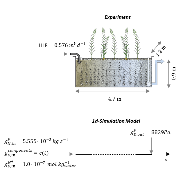
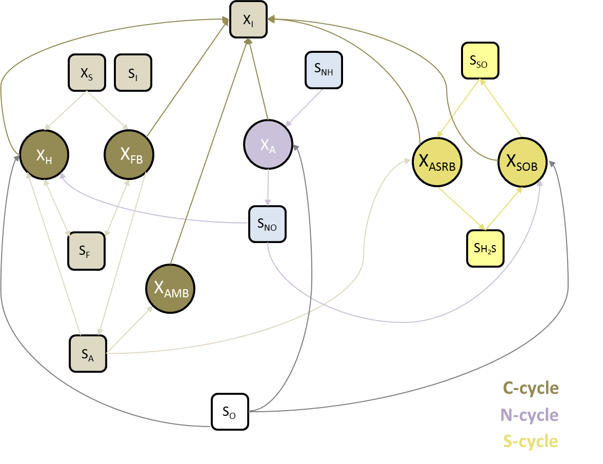
The microbiological processes are modeled by a complex network of kinetic reactions based on the Constructed Wetland Model No. 1 (CWM1) described in Langergraber (2009). The network includes dissolved oxygen ($So$) and nine different soluble and particulated components (“pollutants”) that some of them can be metabolized by six bacterial groups resulting in 17 kinetic reactions (Figure 2). A “clean” system is assumed at start-up in the basin, therefore, initial concentrations of all components (oxygen + “pollutants”) and bacteria are set to 1.0e-4 and 1.0e-3 mg L$^-1$, respectively. For the wastewater components (“pollutants” and oxygen) entering the system, time-dependent Dirichlet BC are defined at the influx point. Respective material properties, initial and boundary conditions are listed in Table 1–2.
 {width=60%}
| Parameter | Description | Value | Unit |
|---|---|---|---|
| Influent & effluent zone | |||
| $\phi$ | Porosity | 0.38 | - |
| $\kappa$ | Permeability | 1.0e-7 | m$^2$ |
| $S$ | Storage | 0.0 | - |
| $a_L$ | long. Dispersion length | 0.45 | m |
| Treatment zone | |||
| $\phi$ | Porosity | 0.38 | - |
| $\kappa$ | Permeability | 1.0e-8 | m$^2$ |
| $S$ | Storage | 0.0 | - |
| $a_L$ | long. Dispersion length | 0.40 | m |
Table 1: Media, material and component properties
| Parameter | Description | Value | Unit |
|---|---|---|---|
| $p(t=0)$ | Initial pressure | 8829 | Pa |
| $g_{N,in}^p$ | Water influx | 5.555e-3 | kg s$^{-1}$ |
| $g_{D,out}^p$ | Pressure at outlet | 8829 | Pa |
| $c_{components}(t=0)$ | Initial component concentrations | 1.0e-4 | g kg$^{-1}$ water |
| $c_{bacteria}(t=0)$ | Initial bacteria concentrations | 1.0e-3 | g kg${^-1}$ water |
| $c_{\text{H}^+}(t=0)$ | Initial concentration of $\text{H}^+$ | 1.0e-7 | mol kg${^-1}$ water |
| $g_{D,in}^{components_c}$ | Influent component concentrations | $f(t)$ | g kg${^-1}$ water |
| $g_{D,in}^{\text{H}^+}$ | Influent concentration of $\text{H}^+$ | 1.0e-7 | mol kg${^-1}$ water |
Table 2: Initial and boundary conditions
Results
Influent wastewater components (oxygen and pollutants) spread through the model domain by advective–dispersive transport (Figure 3). The aeration increases dissolved oxygen concentration $S_O$ in the entire domain. After 2.5 days (2.16e+5 seconds), rapidly growing heterotrophic bacteria $X_H$ starts to consume available $S_O$ and influent organic carbon ($S_A$, $S_F$). Initial growth of $X_H$ and the high concentrations of organic carbon sources at the influent region result in an oxygen depletion. This triggers the growth of anaerobic fermenting bacteria $X_{FB}$ at the front and pushes $X_H$ downstream were enough $S_O$ is available. After organic carbon concentration profiles of $S_F$ and $S_A$ stabilized, autotrophic nitrifying bacteria $X_A$ starts to grow by oxidizing available ammonia ($S_{NH}$) to nitrate/nitrite $S_{NO}$. After 20 days (1.7286e+6 seconds) the microbial reaction network in the wetland has reached a quasi steady–state. The biochemical reactions are now governing the system behaviour.
Both, OGS-6 and OGS-5 simulations yield the same results. For instance, the difference between the OGS-6 and the OGS-5 computation for the concentration of $S_A$ expressed as root mean squared error is 1.11e-4 g L$^{-1}$ (over all time steps and mesh nodes); the corresponding relative mean squared error is 0.37%. The relatively high error may be associated with the missing transport or charge in the OGS-6 simulation, which affects computations by PHREEQC. Please note that due to the long computation time of the simulation (~13 h), the corresponding test (Wetland_1d.prj) is reduced to the first four time steps (28800 s).
Simulated concentrations of solutes (left) and bacteria (right). Solid lines represent solutions by OGS-5; dashed lines represent solution by OGS-6.
References
Boog, J., Kalbacher, T., Nivala, J., Forquet, N., van Afferden, M., Müller, R.A., 2019. Modeling the relationship of aeration, oxygen transfer and treatment performance in aerated horizontal flow treatment wetlands. Water Research. 157 , 321 - 334. https://doi.org/10.1016/j.watres.2019.03.062.
Langergraber, G., Rousseau, D.P.L., García, J., Mena, J., 2009. CWM1: A general model to describe biokinetic processes in subsurface flow constructed wetlands. Water Science and Technology, 59 (9), 1687-1697. https://doi.org/10.2166/wst.2009.131.
This article was written by Johannes Boog. If you are missing something or you find an error please let us know.
Generated with Hugo 0.147.9
in CI job 683680
|
Last revision: December 20, 2025
Commit: chore: fix spelling mistakes fbc5f730
| Edit this page on