Decay-chain problem
![]() This page is based on a Jupyter notebook.
This page is based on a Jupyter notebook.


Decay-chain problem
Problem description
This benchmark is meant to model the diffusive migration of the radionuclides of a simplified Curium-247 decay chain through a semi-infinite porous media column (1-D). The diagram below shows the simplified Curium-247 decay chain which contains 6 radionuclides ending with Actinium-227. All following nuclides have half-lives below 20 a and are neglected for this benchmark.
import os…
(click to toggle)
import os
import time
from pathlib import Path
from subprocess import run

import DecayChainAnalytical as ana
import h5py
import matplotlib.pyplot as plt
import numpy as np
import ogstools as otActinium decay chain A = 4n + 3
According to the mass conservation law, the reactive-diffusive transport of each member of the simplified Curium-247 decay chain can be described by:
$$ \frac{\partial \left( \phi c_{i} \right)}{\partial t} = \nabla \cdot \left(\phi \mathrm{D_p} \nabla c_{i} \right) + \phi k_{i-1} c_{i-1} - \phi k_{i} c_{i}, \quad \forall i = 1,2,...,n, $$where $c_{i}$ [mol/m$^3$] is the concentration of radionuclide $i$, $\phi$ [-] is the porosity, $\mathrm{D_p}$ [m$^2$/s] is the pore diffusion coefficient, and $k_{i}$ [1/s] is the first-order decay constant of a radionuclide $i$, i.e.:
$$ k_i = \mathrm{ln} 2 \, / \, t_{i,1/2}, $$where $t_{i,1/2}$ [s] is its half life.
Model setup
porosity = 0.12
diffusion_constant = 1e-11
# Diffusion coefficient [m2/s]…
(click to toggle)
# Diffusion coefficient [m2/s]
D = 1e-11
# Pore water velocity [m/s]
v = 0
# Half life [year]
radionuclides = np.array(
    ["[Cm-247]", "[Am-243]", "[Pu-239]", "[U-235]", "[Pa-231]", "[Ac-227]"]
)
half_lifes = np.array([1.56e7, 7.37e3, 2.41e4, 7.04e8, 3.28e4, 21.773])
# First-order decay constant [1/s]
k = {
    radionuclide: np.log(2) / half_life / 3.1536e7
    for radionuclide, half_life in zip(radionuclides, half_lifes, strict=True)
}

###Initial and boundary conditions###
c_inlet = np.ones(6)

###Spatial and temporal discretization###
# Distance [m]
dx = np.logspace(-3, 0, 2000)
x = np.hstack(([0], np.cumsum(dx)))
x *= 20 / x[-1]
assert x[-1] == 20  # end point of the 1D mesh
assert x[0] == 0  # start point of the 1D mesh
assert abs(np.min(np.diff(x))) < 1e-3  # minimum cell size of the 1D mesh
assert abs(np.max(np.diff(x))) < 1e-1  # maximum cell size of the 1D mesh
assert np.all(np.diff(x, n=2) > 0)  # monotonically increasing cell sizes

# Time [year]
t = 1e5In the 1-D model, the computational domain is set to be 20 meters long, which is sufficient to ensure that the concentration profile does not reach the right-hand-side boundary during simulation. The simulated time is 100 000 years. Initially, the entire domain is assumed to be solute free, i.e., $c_{\mathrm{ini}}(x, 0) = 0$ mol/m$^3$. The inlet concentration for all the radionuclides is fixed to 10$^{-3}$ mol/m$^3$ throughout the simulated time, i.e., $c(0, t) = 1$ mol/L. The spatial domain is discretized by linear line elements and the grid near the inlet is refined in order to achieve sufficiently high accuracy. A fixed time step size of one hundred years is used in the simulation. The linearized governing equation system is iteratively solved using the standard Picard iteration method.
The table below summarizes the transport parameters and spatio-temporal discretization parameters used in the simulation.
| Parameter | Value | Unit |
|---|---|---|
| Porosity $\phi$ | 0.12 | - |
| Pore diffusion coefficient $\mathrm{D_p}$ | 1e-11 | m$^2$/s |
| Time step size $\Delta t$ | 1e2 | year |
| Grid size $\Delta x$ | 0.00512 - 1.985 | m |
The following table lists the dataset for the half-life of the radionuclides
| Radionuclide | Half-life [year] | First-order decay constant [1/year] |
|---|---|---|
| Cm-247 | 1.56$\times$10$^{7}$ | 4.44$\times$10$^{-8}$ |
| Am-243 | 7.37$\times$10$^{3}$ | 9.40$\times$10$^{-5}$ |
| Pu-239 | 2.41$\times$10$^{4}$ | 2.88$\times$10$^{-5}$ |
| U-235 | 7.04$\times$10$^{8}$ | 9.84$\times$10$^{-10}$ |
| Pa-231 | 3.28$\times$10$^{4}$ | 2.11$\times$10$^{-5}$ |
| Ac-227 | 21.773 | 3.18$\times$10$^{-2}$ |
Notes: The half-life dataset is sourced from Report GRS-289.
Results
Analytical solution
The analytical solution for the reactive-diffusive transport of radionuclides makes use of an expression for the reactive part developed by Sun et al. (1999) for linear reaction chains by making use of an auxiliary varibale $a_i$ and replacing $c_i$ by:
$$ c_{i} = a_{i} - \sum_{j=1}^{i-1} \prod_{l=j}^{i-1} \frac{k_{l}}{k_{l} - k_{i}} c_{j}, \quad \forall i = 2,3,...,n, $$in an otherwise defined analytical solution for transport.
Concentration profiles
c = ana.computeConcentrations(x, t, v, D, k, radionuclides, c_inlet)…
(click to toggle)
c = ana.computeConcentrations(x, t, v, D, k, radionuclides, c_inlet)

fig, ax = plt.subplots()
colors = plt.cm.rainbow(np.linspace(0, 1, radionuclides.size))

for rn, color in zip(radionuclides, colors, strict=True):
    ax.plot(x, c[rn], "-", lw=1.5, label=str(rn), c=color, zorder=10, clip_on=False)

ax.legend(frameon=True, loc="upper right", numpoints=1, fontsize=12, ncol=1)
ax.set(xlim=(0, 20), ylim=(0, 1.4))
ax.set(xlabel="Distance [m]", ylabel="Concentration [mol/L]")
ax.grid(which="both", color="gray", linestyle="dashed")

Concenctration gradient
x_mid = 0.5 * (x[:-1] + x[1:])…
(click to toggle)
x_mid = 0.5 * (x[:-1] + x[1:])
grad_c = ana.computeGradients(x_mid, t, v, D, k, radionuclides, c_inlet)
grad_c_num = {n: (cs[1:] - cs[:-1]) / np.diff(x) for n, cs in c.items()}The following graph is just a self-check that the derived analytical expression for the gradient of the analytical solution is correct. The left plot shows both the analytical and numerical (central differences) gradient of the analytical solution for all nuclide concentrations. The center plot shows the difference between analytical and numerical gradients, and the right one the difference normalized to the range in which the numerical gradient varies. This normalized error is smaller than $10^{-6}$ for all nuclides.
fig, axs = plt.subplots(1, 3, sharex=True)…
(click to toggle)
fig, axs = plt.subplots(1, 3, sharex=True)

for name, color in zip(radionuclides, colors, strict=True):
    grad_cs = grad_c[name]
    grad_cs_num = grad_c_num[name]
    delta_grad_cs = grad_cs - grad_cs_num
    delta_grad_cs_normalized = delta_grad_cs / np.ptp(grad_cs_num)

    np.testing.assert_array_less(np.abs(delta_grad_cs), 3.5e-6)
    np.testing.assert_array_less(np.abs(delta_grad_cs_normalized), 9e-7)

    axs[0].plot(x_mid, grad_cs, label=name, color=color)
    axs[0].plot(x_mid, grad_cs_num, ls=":", color=color, lw=3)
    axs[1].plot(x_mid, grad_cs - grad_cs_num, color=color)
    axs[2].plot(x_mid, delta_grad_cs_normalized, color=color)


axs[0].set_xlabel("$x$ / m")
axs[0].set_ylabel(r"$\mathrm{grad}\;c$ / mol L$^{-1}$ m$^{-1}$")
axs[1].set_ylabel(r"$\mathrm{grad}\;c$ error / mol L$^{-1}$ m$^{-1}$")
axs[2].set_ylabel(r"normalized $\mathrm{grad}\;c$ error / 1")

axs[0].set_title(
    rf"$\mathrm{{grad}}\,c$ of the analytical solution at $t = {t:.0g}\,\mathrm{{years}}$"
)
axs[1].set_title(r"Difference between analytical and numerical $\mathrm{grad}\,c$")
axs[2].set_title(r"Normalized $\mathrm{grad}\,c$ difference")

axs[0].set_ylim(-0.5, 0.2)
axs[0].plot([], [], ":k", lw=3, label="numerical")
axs[0].legend()

fig.set_size_inches(18, 5)
fig.subplots_adjust(wspace=0.25)

Numerical solution
Run simulations
Two numerical models are presented here, one based on the global implicit approach (GIA) and the other on the operator splitting approach (OS). The OGS input files of these two models can be found here. Then, the obtained numerical solutions both are plotted against the analytical solution for verification.
###Run two numerical models###…
(click to toggle)
###Run two numerical models###
prj_name = "1d_decay_chain"
prj_file_GIA = Path(f"./GlobalImplicitApproach/{prj_name}_GIA.prj")
prj_file_OS = Path(f"./{prj_name}_OS.prj")

out_dir = Path(os.environ.get("OGS_TESTRUNNER_OUT_DIR", "_out"))
out_dir.mkdir(parents=True, exist_ok=True)
start_time = time.time()…
(click to toggle)
start_time = time.time()
run(
    f"ogs -o {out_dir} {prj_file_GIA} > {out_dir}/out.txt",
    shell=True,
    check=True,
)
end_time = time.time()
runtime_GIA = round(end_time - start_time, 2)
print("Execution time for the GIA model is ", runtime_GIA, "s")Execution time for the GIA model is 19.2 s
Concentration profiles
ms_GIA = ot.MeshSeries(f"{out_dir}/{prj_name}_GIA.pvd")…
(click to toggle)
ms_GIA = ot.MeshSeries(f"{out_dir}/{prj_name}_GIA.pvd")
assert np.isclose(ms_GIA.timevalues[-1], t * 3.1536e7)
mesh_GIA = ms_GIA[-1].clip("x", origin=(20, 0, 0))
GIA_x = mesh_GIA.points[:, 0]
# Given the fact that the runtime of the OS model (about 1800s) is
# far longer than the time constraint specified (600s), we decide not
# to use the OS simulation results obtained from automated testing.
# Instead, the pre-prepared reference simulation results are used.
ms_OS = ot.MeshSeries(f"{prj_name}_OS.pvd")
mesh_OS = ms_OS[-1].clip("x", origin=(20, 0, 0))
assert np.isclose(ms_OS.timevalues[-1], t * 3.1536e7)
OS_x = mesh_OS.points[:, 0]
def clip_data(x_, y_, x_lim=0.6):
return (x_[np.where(x_ < x_lim)], y_[np.where(x_ < x_lim)])
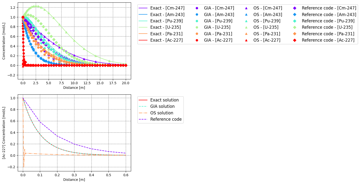
fig, axs = plt.subplots(1, 2, figsize=(14, 5), sharey=True)
axs[0].set(xlabel="Distance [m]", ylabel="Concentration [mol/L]")
axs[1].set(xlabel="Distance [m]", ylabel="[Ac-227] Concentration [mol/L]")
axs[1].plot(*clip_data(x, c["[Ac-227]"]), "-k", lw=1.5, label="Exact", zorder=10)
axs[1].plot(*clip_data(GIA_x, mesh_GIA["[Ac-227]"]), "--or", lw=1.5, label="OGS GIA")
axs[1].plot(*clip_data(OS_x, mesh_OS["[Ac-227]"]), "-.^r", lw=1.5, label="OGS OS")
for rn, color in zip(radionuclides, colors, strict=True):
c_gia = mesh_GIA[rn]
c_os = mesh_OS[rn]
axs[0].plot(x, c[rn], "-", lw=1.5, label=rn, c=color)
axs[0].plot(GIA_x, c_gia, "o", color=color, markevery=50)
axs[0].plot(OS_x, c_os, "^", color=color, markevery=50)
# numerical solution by reference code
# added once the bc value is double-checked
with h5py.File("./solution_reference_code.hdf5", "r") as f:
for s_, color in zip(f["species"][:], colors, strict=True):
value = f[s_][:, 1] / porosity
axs[0].plot(f["x"][:], value, "D", color=color, markevery=5, fillstyle="none")
if s_ == b"Ac-227":
axs[1].plot(
*clip_data(f["x"][:], value), ":Dr", label="Reference", fillstyle="none"
)
axs[0].grid(which="both", color="gray", linestyle="dashed")
axs[1].grid(which="both", color="gray", linestyle="dashed")
axs[0].plot([], [], "-k", lw=1.5, label="Exact")
axs[0].plot([], [], "ok", label="OGS GIA")
axs[0].plot([], [], "^k", label="OGS OS")
axs[0].plot([], [], "Dk", fillstyle="none", label="Reference code")
axs[0].legend()
_ = axs[1].legend()

As can be seen from Subfigure 1, for all radionuclides except the fastest decaying Actinium-227, the predicted concentration profiles using GIA and OS both agree well with the analytical solutions. For Actinium-227 concentration, the GIA solution perfectly matches with the reference result (see Subfigure 2). By contrast, the OS solution near the inlet deviates significantly from the reference result. The observed deviation is due to the fact that the time step size adopted in the simulation ($\Delta t$ = 100 years) is too large compared to the half-life of Actinium-227 ($t_{1/2}$ = 21.773 years).
Molar fluxes (GIA simulation)
The following graph shows the molar fluxes obtained both analytically (solid lines) and numerically (GIA approach, thick, dotted lines). It can be seen that both results coincide well.
grad_c = ana.computeGradients(x, t, v, D, k, radionuclides, c_inlet)…
(click to toggle)
grad_c = ana.computeGradients(x, t, v, D, k, radionuclides, c_inlet)
molar_flux_ana = {
    n: -porosity * diffusion_constant * grad_cs for n, grad_cs in grad_c.items()
}

fig, ax = plt.subplots()
ax.axhline(0, ls=":", color="gray")
ax.set_title(rf"Molar fluxes after $t = {t:.0g}\,\mathrm{{years}}$")
ax.set(xlabel="$x$ / m", ylabel="molar flux / mol L$^{-1}$ m s$^{-1}$")

for rn, color in zip(radionuclides, colors, strict=True):
    ax.plot(x, molar_flux_ana[rn], "-", lw=1.5, label=f"Analytical – {rn}", c=color)
    ax.plot(GIA_x, mesh_GIA[rn + "Flux"], ":", lw=3, c=color)

ax.set(xlim=(-0.1, 20), ylim=(-3e-13, 8e-13))
ax.plot([], [], ":k", lw=3, label="Numerial (OGS GIA)")
ax.legend()<matplotlib.legend.Legend at 0x7fa4e18539d0>

Error analysis
Furthermore, we perform an error analysis of the GIA and OS solutions. As can be observed from Subfigures 1 and 3, the absolute error of the GIA solution for all the radionuclides is suppressed at a low level. The maximum absolute error is only $3.6 \cdot 10^{-4}$ mol/L. In contrast, the absolute error of the OS solution is two to three orders of magnitude greater than that of the GIA solution (see Subfigures 2 and 3). And the error becomes more apparent closer to the inlet.
fig, axs = plt.subplots(3, 1, figsize=(5, 13.5))…
(click to toggle)
fig, axs = plt.subplots(3, 1, figsize=(5, 13.5))

for rn, color in zip(radionuclides, colors, strict=True):
    delta_GIA = np.abs(mesh_GIA[rn] - np.interp(GIA_x, x, c[rn]))
    delta_OS = np.abs(mesh_OS[rn] - np.interp(OS_x, x, c[rn]))

    np.testing.assert_array_less(delta_GIA, 3.6e-4)

    axs[0].plot(GIA_x, delta_GIA, "-", color=color, label=f"OGS GIA {rn}")
    if rn == "[Ac-227]":
        np.testing.assert_array_less(delta_OS, 1.2)
        axs[2].plot(*clip_data(GIA_x, delta_GIA), "-r", label=f"OGS GIA {rn}")
        axs[2].plot(*clip_data(OS_x, delta_OS), "--r", label=f"OGS OS {rn}")
    else:
        np.testing.assert_array_less(delta_OS, 0.012)
        axs[1].plot(OS_x, delta_OS, "--", color=color, label=f"OGS OS {rn}")

for i in range(3):
    axs[i].set(xlabel="Distance [m]", ylabel="Concentration error [mol/L]")
    axs[i].grid(which="both", color="gray", linestyle="dashed")
    _ = axs[i].legend()

Molar fluxes
The following plots show the difference between numerically computed molar fluxes (OGS, GIA approach) and analytically derived fluxes (left plot), and that difference normalized to the range of analytical concentration gradients (right plot). That normalized error is smaller than 0.1 % for all nuclides.
fig, axs = plt.subplots(1, 2, figsize=(12, 5), sharex=True)…
(click to toggle)
fig, axs = plt.subplots(1, 2, figsize=(12, 5), sharex=True)
axs: list[plt.Axes]
axs[0].set(xlabel="$x$ / m", ylabel=r"molar flux error / mol L$^{-1}$ m s$^{-1}$")
axs[1].set(xlabel="$x$ / m", ylabel=r"normalized molar flux error / 1")
axs[0].set_title(
    rf"Molar flux error (GIA – analytical) after $t = {t:.0g}\,\mathrm{{years}}$"
)
axs[1].set_title(r"Normalized molar flux error")
axs[0].set_yscale("asinh", linear_width=5e-18)
axs[1].set_yscale("asinh", linear_width=1e-4)

for rn, color in zip(radionuclides, colors, strict=True):
    flux_err = np.interp(x, GIA_x, mesh_GIA[rn + "Flux"]) - molar_flux_ana[rn]
    flux_err_normalized = flux_err / np.ptp(molar_flux_ana[rn])
    np.testing.assert_array_less(np.abs(flux_err_normalized)[x > GIA_x[1]], 8e-4)

    axs[0].plot(x, flux_err, label=rn, color=color)
    axs[1].plot(x, flux_err_normalized, label=rn, color=color)

for ax in axs:
    ax.set_xlim((0.5 * GIA_x[1], 1.5 * x[-1]))
    ax.autoscale(False)
    marker_y = [ax.get_ylim()[0]] * len(GIA_x)
    ax.scatter(GIA_x, marker_y, c="k", marker="|", alpha=0.5, label="OGS mesh nodes")
    ax.axvspan(0.5 * GIA_x[1], GIA_x[1], alpha=1, color="0.9")
    ax.axvspan(x[-1], 1.5 * x[-1], alpha=1, color="0.9")
    ax.set_xscale("log")
    ax.grid(which="minor", color="0.95")
    ax.grid(which="major", color="lightgray")
    ax.legend()

Molar fluxes are a secondary quantity in OGS. They are computed at the integration points of each mesh element and extrapolated to the mesh nodes for output purposes. The contributions to the nodal values from each adjacent mesh element are averaged. This extrapolation and averaging procedure leads to errors itself. OGS computes an error indicator for the extrapolation and averaging error. This indicator is the root mean square error when re-interpolating the extrapolated and averaged molar fluxes back to the integration points. It is computed as a cell field. It is shown for all nuclides in the plots below. The left plot shows the extrapolation residuals, the right one the extrapolation residuals normalized to the range of molar fluxes. That normalized error is smaller than 0.23 % for all nuclides but Ac-227, for which it is smaller than 1.5 %. The error estimate is larger — in the Ac-227 case much larger — than the actual error. I.e., in this case, it is a conservative estimate of the actual error, but it’s worthwhile to reconsider this on a case-by-case basis.
###Read simulation results###…
(click to toggle)
###Read simulation results###

mesh_GIA = ms_GIA[-1].clip("x", origin=(50, 0, 0))
GIA_x = mesh_GIA.points[:, 0]
GIA_center_x = mesh_GIA.cell_centers(vertex=False).points[:, 0]
assert np.all(np.diff(GIA_center_x) > 0)
grad_c_ex = ana.computeGradients(GIA_center_x, t, v, D, k, radionuclides, c_inlet)
molar_flux_ana_ex = {
    n: -porosity * diffusion_constant * grad_cs for n, grad_cs in grad_c_ex.items()
}

fig, axs = plt.subplots(1, 2, figsize=(12, 5), sharex=True)
axs: list[plt.Axes]
axs[0].set_ylabel(
    r"molar flux extrapolation residual / mol L$^{-1}$ m s$^{-1}$",
)
axs[1].set_ylabel(r"normalized extrapolation residual / 1")
axs[0].set_title(
    rf"OGS molar flux extrapolation residual after $t = {t:.0g}\,\mathrm{{years}}$"
)
axs[1].set_title(r"Normalized extrapolation residual")

for rn, color in zip(radionuclides, colors, strict=True):
    flux_res = mesh_GIA[rn + "Flux_residual"]
    flux_res_normalized = flux_res / np.ptp(molar_flux_ana_ex[rn])
    if rn != "[Ac-227]":
        np.testing.assert_array_less(np.abs(flux_res_normalized), 0.0023)
    np.testing.assert_array_less(np.abs(flux_res_normalized), 1.5e-2)

    axs[0].loglog(GIA_center_x, flux_res, label=rn, color=color)
    axs[1].loglog(GIA_center_x, flux_res_normalized, label=rn, color=color)

for ax in axs:
    ax.set_xlim((0.75 * GIA_x[1], 1.5 * GIA_x[-1]))
    ax.autoscale(False)
    marker_y = [ax.get_ylim()[0]] * len(GIA_x)
    ax.scatter(GIA_x, marker_y, c="k", marker="|", alpha=0.5, label="OGS mesh nodes")
    ax.set_xlabel("$x$ / m")
    ax.grid(which="minor", color="0.95")
    ax.grid(which="major", color="lightgray")
    ax.legend()

The effect of time step size
As shown in the figure below, the OS solution is rather sensitive to the time stepping scheme. By reducing the time step size from 100 years to 5 years, the solution accuracy near the inlet is greatly improved. Nevertheless, the OS solution accuracy is yet lower than that of the GIA solution despite a larger time step size.
ms_OS_5a = ot.MeshSeries(f"{prj_name}_OS_5year.pvd")…
(click to toggle)
ms_OS_5a = ot.MeshSeries(f"{prj_name}_OS_5year.pvd")
assert np.isclose(ms_OS_5a.timevalues[-1], t * 3.1536e7)
mesh_OS_5a = ms_OS_5a[-1].clip("x", origin=(0.6, 0, 0))
OS_5a_x = mesh_OS_5a.points[:, 0]

fig, ax = plt.subplots()

ac = radionuclides[-1]
ax.plot(x, c[ac], "-", lw=1.5, label="Exact")
ax.plot(OS_x, mesh_OS[ac], "--", lw=1.5, label=r"$\Delta$t = 100 years")
ax.plot(OS_5a_x, mesh_OS_5a[ac], "-.", lw=1.5, label=r"$\Delta$t = 5 years")

ax.legend(frameon=True, loc="upper right", fontsize=12)
ax.set(xlim=(-0.025, 0.6))
ax.set(xlabel="Distance [m]", ylabel=f"{ac} Concentration [mol/L]")
ax.grid(which="both", color="gray", linestyle="dashed")
Computational performance of two solution strategies
The runtime of the GIA model is only 22.13 seconds, approximately two orders of magnitude faster than the OS model in this case (see the figure below). Further time profiling analysis for the OS model indicates that PHREEQC consumes over 90 percent of the runtime for solving the local decay-chain problem. To summarize, the global implicit approach (GIA) is clearly superior to the operator splitting approach in terms of solution accuracy and computational performance. Moreover, the global implicit approach even allows for a larger time step size.
The effect of parallelization on computational performance
In order to further improve the computational performance of the GIA model, MPI parallelization is employed. As its result, the simulation runtime is drastically reduced down to 4.82 seconds with the number of processors increased to 8. This results in a 4.6X speed boost.
runtimes = {"OS - 1 Processor": 1980, "GIA - 1 Processor": runtime_GIA}…
(click to toggle)
runtimes = {"OS - 1 Processor": 1980, "GIA - 1 Processor": runtime_GIA}
for n in [4, 8]:
    prj_GIA_np = Path(f"./GlobalImplicitApproach/MPI/{n}Processors/{prj_name}_GIA.prj")

    cmd = f"mpirun --bind-to none -np {n} ogs {prj_GIA_np} -o {out_dir} > {out_dir}/out.txt"
    print(cmd)
    start_time = time.time()
    run(cmd, shell=True, check=True)
    end_time = time.time()
    runtimes[f"GIA - {n} Processors"] = round(end_time - start_time, 2)
    print(
        f"Execution time for the parallelized GIA model with {n} processors is ",
        runtimes[f"GIA - {n} Processors"],
        "s",
)mpirun --bind-to none -np 4 ogs GlobalImplicitApproach/MPI/4Processors/1d_decay_chain_GIA.prj -o /var/lib/gitlab-runner/builds/vZ6vnZiU/0/ogs/build/release-petsc/Tests/Data/Parabolic/ComponentTransport/ReactiveTransport/DecayChain/DecayChain > /var/lib/gitlab-runner/builds/vZ6vnZiU/0/ogs/build/release-petsc/Tests/Data/Parabolic/ComponentTransport/ReactiveTransport/DecayChain/DecayChain/out.txt
Execution time for the parallelized GIA model with 4 processors is  9.77 s
mpirun --bind-to none -np 8 ogs GlobalImplicitApproach/MPI/8Processors/1d_decay_chain_GIA.prj -o /var/lib/gitlab-runner/builds/vZ6vnZiU/0/ogs/build/release-petsc/Tests/Data/Parabolic/ComponentTransport/ReactiveTransport/DecayChain/DecayChain > /var/lib/gitlab-runner/builds/vZ6vnZiU/0/ogs/build/release-petsc/Tests/Data/Parabolic/ComponentTransport/ReactiveTransport/DecayChain/DecayChain/out.txt
Execution time for the parallelized GIA model with 8 processors is 14.33 s
fig, axs = plt.subplots(1, 2, figsize=(12, 5))…
(click to toggle)
fig, axs = plt.subplots(1, 2, figsize=(12, 5))
for i, stop in enumerate([2, None]):
    axs[i].set_ylabel("Runtime [second]")
    axs[i].yaxis.grid(color="gray", linestyle="dashed", zorder=0)
    axs[i].margins(y=0.2)

    for j, (k, v) in enumerate(list(runtimes.items())[i:stop]):
        color = f"C{3-list(runtimes).index(k)}"
        axs[i].bar(k, v, width=0.5, zorder=3, color=color)
        axs[i].annotate(v, (j, v + [50, 1][i]), ha="center")

References
(GRS 289) VSG: Radiologische Konsequenzenanalyse (AP 10). J. Larue, B. Baltes, H. Fischer, G. Frieling, I. Kock, M. Navarro, H. Seher.
Sun, Y., Petersen, J. N., & Clement, T. P. (1999). Analytical solutions for multiple species reactive transport in multiple dimensions. Journal of Contaminant Hydrology, 35(4), 429-440.
Credits:
Renchao Lu, Christoph Behrens, Dmitri Naumov, Christoph Lehmann, Haibing Shao
This article was written by Renchao Lu, Christoph Behrens, Dmitri Naumov, Christoph Lehmann, Haibing Shao. If you are missing something or you find an error please let us know.
Generated with Hugo 0.150.1
in CI job 743172
|
Last revision: August 5, 2022