Surfing boundary
![]() This page is based on a Jupyter notebook.
This page is based on a Jupyter notebook.


Problem description
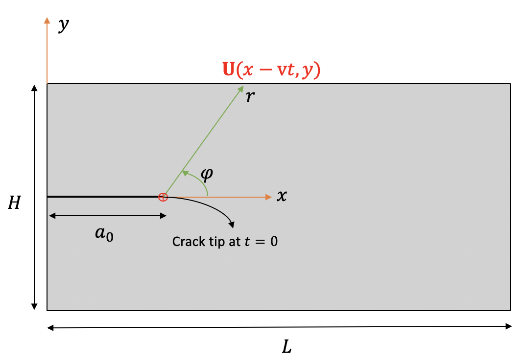
Consider a plate, $\Omega=[0,2]\times [-0.5,0.5]$, with an explicit edge crack, $\Gamma=[0,0.5]\times \{0\}$; that is subjected to a time dependent crack opening displacement:
\begin{eqnarray} \label{eq:surfing_bc} \mathbf{u}(x,y,t)= \mathbf{U}(x-\text{v}t,y) \quad \text{on} \quad \partial\Omega_D, \end{eqnarray} where $\text{v}$ is an imposed loading velocity; and $\mathbf{U}$ is the asymptotic solution for the Mode-I crack opening displacement \begin{eqnarray} \label{eq:asymptotic} U_x= \dfrac{K_I}{2\mu} \sqrt{\dfrac{r}{2\pi}} (\kappa-\cos \varphi) \cos \frac{\varphi}{2}, \nonumber \ U_y= \dfrac{K_I}{2\mu} \sqrt{\dfrac{r}{2\pi}} (\kappa-\cos \varphi) \sin \frac{\varphi}{2}, \end{eqnarray}
where $K_I$ is the stress intensity factor, $\kappa=(3-\nu)/(1+\nu)$ and $\mu=E / 2 (1 + \nu) $; $(r,\varphi)$ are the polar coordinate system, where the origin is crack tip. Also, we used $G_\mathrm{c}=K_{Ic}^2(1-\nu^2)/E$ as the fracture surface energy under plane strain condition. Table 1 lists the material properties and geometry of the numerical model.
Input Data
| Name | Value | Unit | Symbol |
|---|---|---|---|
| Young’s modulus | 210x$10^3$ | MPa | $E$ |
| Critical energy release rate | 2.7 | MPa$\cdot$mm | $G_{c}$ |
| Poisson’s ratio | 0.3 | $-$ | $\nu$ |
| Regularization parameter | 2$h$ | mm | $\ell_s$ |
| Imposed loading velocity | 1.5 | mm/s | $\text{v}$ |
| Length | $2$ | mm | $L$ |
| Height | $1$ | mm | $H$ |
| Initial crack length | $0.5$ | mm | $a_0$ |
x_tip_Initial = 0.5
y_tip_Initial = 0.5
Height = 1.0

Orientation = 0
h = 0.05
G_i = 2.7
ls = 2 * h
# We set ls=2h in our simulation
phasefield_model = "AT1" # AT1 and AT2Paths and project file name
import os

# file's name
prj_name = "surfing.prj"

from pathlib import Path

out_dir = Path(os.environ.get("OGS_TESTRUNNER_OUT_DIR", "_out"))
if not out_dir.exists():
out_dir.mkdir(parents=True)Mesh generation
# https://www.opengeosys.org/docs/tools/meshing/structured-mesh-generation/
! generateStructuredMesh -o {out_dir}/surfing_quad_1x2.vtu -e quad --lx 2 --nx {round(2/h)+1} --ly 1 --ny {round(1/h)+1}
! NodeReordering -i {out_dir}/surfing_quad_1x2.vtu -o {out_dir}/surfing_quad_1x2_NR.vtu[2024-07-03 09:55:52.904] [ogs] [[32minfo[m] Mesh created: 924 nodes, 861 elements.
[2024-07-03 09:55:53.294] [ogs] [[32minfo[m] Reordering nodes...
[2024-07-03 09:55:53.295] [ogs] [[32minfo[m] Corrected 0 elements.
[2024-07-03 09:55:53.298] [ogs] [[32minfo[m] VTU file written.
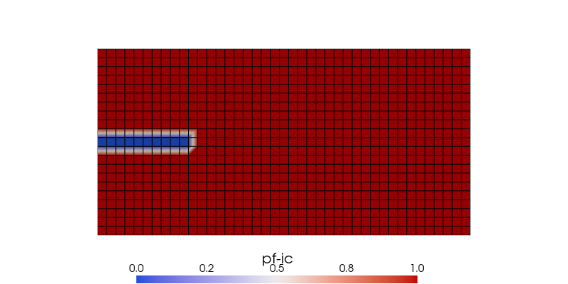
Pre-processing
At fracture, we set the initial phase field to zero.
import pyvista as pv

pv.set_plot_theme("document")
pv.set_jupyter_backend("static")

import numpy as np

mesh = pv.read(f"{out_dir}/surfing_quad_1x2_NR.vtu")
phase_field = np.ones((len(mesh.points), 1))


for node_id, x in enumerate(mesh.points):
    if (
        x[0] < x_tip_Initial + h / 10
        and x[1] < Height / 2 + h
        and x[1] > Height / 2 - h
    ):
        phase_field[node_id] = 0.0

mesh.point_data["pf-ic"] = phase_field
mesh.save(f"{out_dir}/surfing_quad_1x2_NR_pf_ic.vtu")

pf_ic = mesh.point_data["pf-ic"]
sargs = {
    "title": "pf-ic",
    "title_font_size": 20,
    "label_font_size": 15,
    "n_labels": 5,
    "position_x": 0.24,
    "position_y": 0.0,
    "fmt": "%.1f",
    "width": 0.5,
}
clim = [0, 1.0]

p = pv.Plotter(shape=(1, 1), border=False)
p.add_mesh(
    mesh,
    scalars=pf_ic,
    show_edges=True,
    show_scalar_bar=True,
    colormap="coolwarm",
    clim=clim,
    scalar_bar_args=sargs,
)

p.view_xy()
p.camera.zoom(1.5)
p.window_size = [800, 400]
p.show()DRI3 not available
failed to load driver: zink
Run the simulation
from ogs6py import ogs

# Change the length scale and phasefield model in project file
model = ogs.OGS(
    INPUT_FILE=prj_name,
    PROJECT_FILE=f"{out_dir}/{prj_name}",
    MKL=True,
    args=f"-o {out_dir}",
)
model.replace_parameter_value(name="ls", value=2 * h)
model.replace_text(phasefield_model, xpath="./processes/process/phasefield_model")
model.replace_text("./surfing.gml", xpath="./geometry")
model.replace_text("./Surfing_python.py", xpath="./python_script")
model.write_input()

import time

t0 = time.time()
print(">>> OGS started execution ... <<<")
! ogs {out_dir}/{prj_name} -o {out_dir} > {out_dir}/log.txt

tf = time.time()
print(">>> OGS terminated execution <<< Elapsed time: ", round(tf - t0, 2), " s.")>>> OGS started execution ... <<<
>>> OGS terminated execution <<< Elapsed time: 11.34 s.
Results
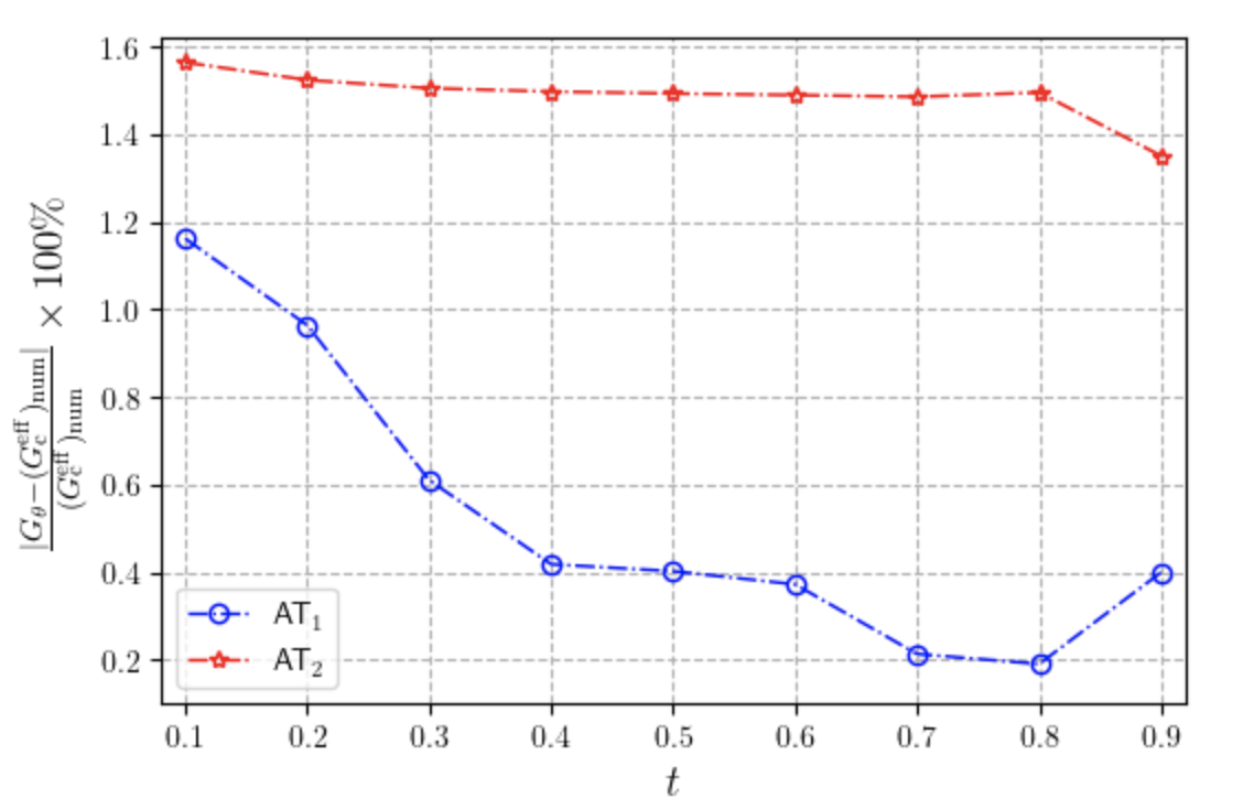
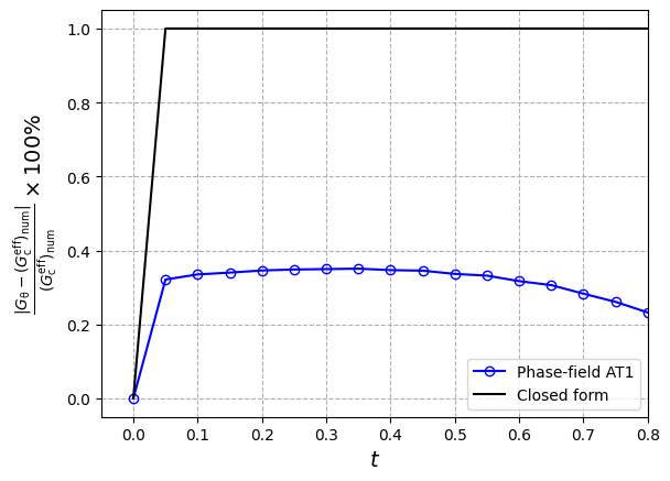
We computed the energy release rate using $G_{\theta}$ method (Destuynder et al., 1983; Li et al., 2016) and plot the errors against the theoretical numerical toughness i.e. $(G_c^{\text{eff}})_{\texttt{num}}=G_c(1+\frac{h}{2\ell})$ for $\texttt{AT}_2$, and $(G_c^{\text{eff}})_{\texttt{num}}=G_c(1+\frac{3h}{8\ell})$ for $\texttt{AT}_1$ (Bourdin et al., 2008).
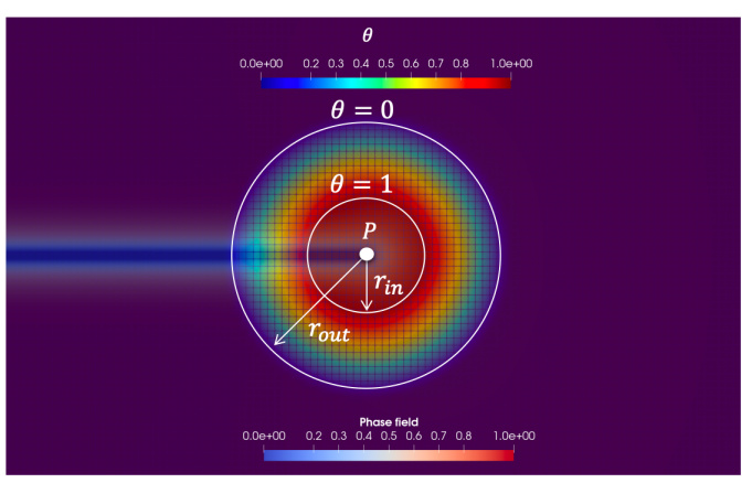
We computed the energy release rate using $G_{\theta}$ method (Destuynder et al., 1983; Li et al., 2016) and plot the errors against the theoretical numerical toughness i.e. $(G_c^{\text{eff}})_{\texttt{num}}=G_c(1+\frac{h}{2\ell})$ for $\texttt{AT}_2$, and $(G_c^{\text{eff}})_{\texttt{num}}=G_c(1+\frac{3h}{8\ell})$ for $\texttt{AT}_1$ (Bourdin et al., 2008).
R_inn = 4 * ls
R_out = 2.5 * R_inn

if phasefield_model == "AT1":
    G_eff = G_i * (1 + 3 * h / (8 * ls))
elif phasefield_model == "AT2":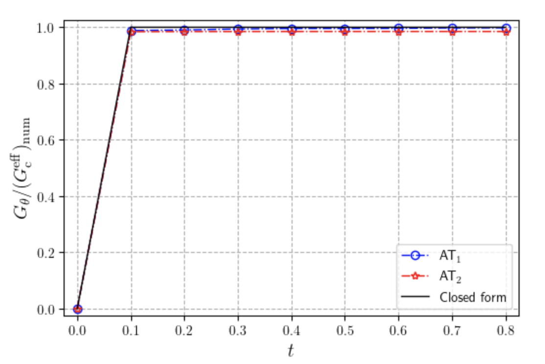
G_eff = G_i * (1 + h / (2 * ls))We run the simulation with a coarse mesh here to reduce computing time; however, a finer mesh would give a more accurate results. The energy release rate and its error for Models $\texttt{AT}_1$ and $\texttt{AT}_2$ with a mesh size of $h=0.005$ are shown below.
Post-processing
from scipy.spatial import Delaunay

reader = pv.get_reader(f"{out_dir}/surfing.pvd")
G_theta_time = np.zeros((len(reader.time_values), 2))


for t, time_value in enumerate(reader.time_values):
    reader.set_active_time_value(time_value)

    mesh = reader.read()[0]
    points = mesh.point_data["phasefield"].shape[0]
    xs = mesh.points[:, 0]
    ys = mesh.points[:, 1]
    pf = mesh.point_data["phasefield"]
    sigma = mesh.point_data["sigma"]
    disp = mesh.point_data["displacement"]

    num_points = disp.shape
    theta = np.zeros(num_points)

    # --------------------------------------------------------------------------------
    # find fracture tip
    # --------------------------------------------------------------------------------
    min_pf = min(pf[:])
    coord_pf_0p5 = mesh.points[pf < 0.5]
    if min_pf <= 0.5:
        coord_pf_0p5[np.argmax(coord_pf_0p5, axis=0)[0]][1]
        x0 = coord_pf_0p5[np.argmax(coord_pf_0p5, axis=0)[0]][0]
        y0 = coord_pf_0p5[np.argmax(coord_pf_0p5, axis=0)[0]][1]
    else:
        x0 = x_tip_Initial
        y0 = y_tip_Initial
    Crack_position = [x0, y0]
    # --------------------------------------------------------------------------------
    # define \theta
    # --------------------------------------------------------------------------------
    for i, x in enumerate(mesh.points):
        # distance from the crack tip
        R = np.sqrt((x[0] - Crack_position[0]) ** 2 + (x[1] - Crack_position[1]) ** 2)
        if R_inn > R:
            theta_funct = 1.0
        elif R_out < R:
            theta_funct = 0.0
        else:
            theta_funct = (R - R_out) / (R_inn - R_out)
        theta[i][0] = theta_funct * np.cos(Orientation)
        theta[i][1] = theta_funct * np.sin(Orientation)

    mesh.point_data["theta"] = theta

    # --------------------------------------------------------------------------------
    # define grad \theta
    # --------------------------------------------------------------------------------
    mesh_theta = mesh.compute_derivative(scalars="theta")
    mesh_theta["gradient"]

    keys = np.array(
        ["thetax_x", "thetax_y", "thetax_z", "thetay_x", "thetay_y", "thetay_z"]
    )
    keys = keys.reshape((2, 3))[:, : mesh_theta["gradient"].shape[1]].ravel()
    gradients_theta = dict(zip(keys, mesh_theta["gradient"].T))
    mesh.point_data.update(gradients_theta)
    # --------------------------------------------------------------------------------
    # define grad u
    # --------------------------------------------------------------------------------
    mesh_u = mesh.compute_derivative(scalars="displacement")
    mesh_u["gradient"]

    keys = np.array(["Ux_x", "Ux_y", "Ux_z", "Uy_x", "Uy_y", "Uy_z"])
    keys = keys.reshape((2, 3))[:, : mesh_u["gradient"].shape[1]].ravel()
    gradients_u = dict(zip(keys, mesh_u["gradient"].T))
    mesh.point_data.update(gradients_u)

    # --------------------------------------------------------------------------------
    # define G_theta
    # --------------------------------------------------------------------------------
    G_theta_i = np.zeros(num_points[0])
    sigma = mesh.point_data["sigma"]
    Ux_x = mesh.point_data["Ux_x"]
    Ux_y = mesh.point_data["Ux_y"]
    Uy_x = mesh.point_data["Uy_x"]
    Uy_y = mesh.point_data["Uy_y"]

    thetax_x = mesh.point_data["thetax_x"]
    thetax_y = mesh.point_data["thetax_y"]
    thetay_x = mesh.point_data["thetay_x"]
    thetay_y = mesh.point_data["thetay_y"]

    for i, _x in enumerate(mesh.points):
        # ---------------------------------------------------------------------------
        sigma_xx = sigma[i][0]
        sigma_yy = sigma[i][1]
        sigma_xy = sigma[i][3]

        Ux_x_i = Ux_x[i]
        Ux_y_i = Ux_y[i]
        Uy_x_i = Uy_x[i]
        Uy_y_i = Uy_y[i]

        thetax_x_i = thetax_x[i]
        thetax_y_i = thetax_y[i]
        thetay_x_i = thetay_x[i]
        thetay_y_i = thetay_y[i]
        # ---------------------------------------------------------------------------
        dUdTheta_11 = Ux_x_i * thetax_x_i + Ux_y_i * thetay_x_i
        dUdTheta_12 = Ux_x_i * thetax_y_i + Ux_y_i * thetay_y_i
        dUdTheta_21 = Uy_x_i * thetax_x_i + Uy_y_i * thetay_x_i
        dUdTheta_22 = Uy_x_i * thetax_y_i + Uy_y_i * thetay_y_i
        trace_sigma_grad_u_grad_theta = (
            sigma_xx * dUdTheta_11
            + sigma_xy * (dUdTheta_12 + dUdTheta_21)
            + sigma_yy * dUdTheta_22
        )
        trace_sigma_grad_u = (
            sigma_xx * Ux_x_i + sigma_xy * (Uy_x_i + Ux_y_i) + sigma_yy * Uy_y_i
        )
        div_theta_i = thetax_x_i + thetay_y_i
        G_theta_i[i] = (
            trace_sigma_grad_u_grad_theta - 0.5 * trace_sigma_grad_u * div_theta_i
        )
    mesh.point_data["G_theta_node"] = G_theta_i
    # --------------------------------------------------------------------------------
    # Integral G_theta
    # --------------------------------------------------------------------------------
    X = mesh.points[:, 0]
    Y = mesh.points[:, 1]
    G_theta_i = mesh.point_data["G_theta_node"]

    domain_points = np.array(list(zip(X, Y)))
    tri = Delaunay(domain_points)

    def area_from_3_points(x, y, z):
        return np.sqrt(np.sum(np.cross(x - y, x - z), axis=-1) ** 2) / 2

    G_theta = 0
    for vertices in tri.simplices:
        mean_value = (
            G_theta_i[vertices[0]] + G_theta_i[vertices[1]] + G_theta_i[vertices[2]]
        ) / 3
        area = area_from_3_points(
            domain_points[vertices[0]],
            domain_points[vertices[1]],
            domain_points[vertices[2]],
        )
        G_theta += mean_value * area
    G_theta_time[t][1] = G_theta
    G_theta_time[t][0] = time_value
mesh.save(f"{out_dir}/surfing_Post_Processing.vtu")Plots
import matplotlib.pyplot as plt

plt.xlabel("$t$", fontsize=14)
plt.ylabel(
    r"$\frac{|{G}_\mathrm{\theta}-({G}_\mathrm{c}^{\mathrm{eff}})_\mathrm{num}|}{({G}_\mathrm{c}^{\mathrm{eff}})_\mathrm{num}}\times 100\%$",
    fontsize=14,
)
plt.plot(
    G_theta_time[:, 0],
    abs(G_theta_time[:, 1]) / G_eff,
    "-ob",
    fillstyle="none",
    linewidth=1.5,
    label="Phase-field %s" % phasefield_model,
)
plt.plot(
    G_theta_time[:, 0],
    np.append(0, np.ones(len(G_theta_time[:, 0]) - 1)),
    "-k",
    fillstyle="none",
    linewidth=1.5,
    label="Closed form",
)
plt.grid(linestyle="dashed")
plt.xlim(-0.05, 0.8)
legend = plt.legend(loc="lower right")
plt.show()

plt.xlabel("$t$", fontsize=14)
plt.ylabel(
    r"$\frac{|{G}_\mathrm{\theta}-({G}_\mathrm{c}^{\mathrm{eff}})_\mathrm{num}|}{({G}_\mathrm{c}^{\mathrm{eff}})_\mathrm{num}}\times 100\%$",
    fontsize=14,
)
plt.plot(
    G_theta_time[:, 0],
    abs(G_theta_time[:, 1] - G_eff) / G_eff * 100,
    "-ob",
    fillstyle="none",
    linewidth=1.5,
    label="Phase-field %s" % phasefield_model,
)
plt.grid(linestyle="dashed")
plt.xlim(-0.05, 0.8)
# plt.ylim(0,4)
legend = plt.legend(loc="upper right")
plt.show()
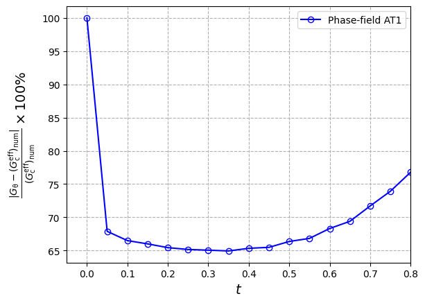
Hint: Accurate results can be obtained by using the mesh size below 0.02.
Phase field profile
Fracture propagation animation
plotter = pv.Plotter()

plotter.open_gif("figures/surfing.gif")
pv.set_plot_theme("document")
for time_value in reader.time_values:
    reader.set_active_time_value(time_value)
    mesh = reader.read()[0]  # This dataset only has 1 block

    sargs = {
        "title": "Phase field",
        "title_font_size": 20,
        "label_font_size": 15,
        "n_labels": 5,
        "position_x": 0.3,
        "position_y": 0.2,
        "fmt": "%.1f",
        "width": 0.5,
    }
    clim = [0, 1.0]
    points = mesh.point_data["phasefield"].shape[0]
    xs = mesh.points[:, 0]
    ys = mesh.points[:, 1]
    pf = mesh.point_data["phasefield"]
    plotter.clear()
    plotter.add_mesh(
        mesh,
        scalars=pf,
        show_scalar_bar=False,
        colormap="coolwarm",
        clim=clim,
        scalar_bar_args=sargs,
        lighting=False,
    )
    plotter.add_text(f"Time: {time_value:.0f}", color="black")

    plotter.view_xy()
    plotter.write_frame()

plotter.close()DRI3 not available
failed to load driver: zink
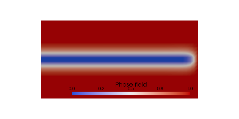
Phase field profile at last time step
mesh = reader.read()[0]

pv.set_jupyter_backend("static")
p = pv.Plotter(shape=(1, 1), border=False)
p.add_mesh(
    mesh,
    scalars=pf,
    show_edges=False,
    show_scalar_bar=True,
    colormap="coolwarm",
    clim=clim,
    scalar_bar_args=sargs,
)

p.view_xy()
p.camera.zoom(1.5)
p.window_size = [800, 400]
p.show()DRI3 not available
failed to load driver: zink
References
[1] B. Bourdin, G.A. Francfort, and J.-J. Marigo, The variational approach to fracture, Journal of Elasticity 91 (2008), no. 1-3, 5–148.
[2] Li, Tianyi, Jean-Jacques Marigo, Daniel Guilbaud, and Serguei Potapov. Numerical investigation of dynamic brittle fracture via gradient damage models. Advanced Modeling and Simulation in Engineering Sciences 3, no. 1 (2016): 1-24.
[3] Dubois, Frédéric and Chazal, Claude and Petit, Christophe, A Finite Element Analysis of Creep-Crack Growth in Viscoelastic Media, Mechanics Time-Dependent Materials 2 (1998), no. 3, 269–286
This article was written by Mostafa Mollaali, Keita Yoshioka. If you are missing something or you find an error please let us know.
Generated with Hugo 0.122.0
in CI job 449919
|
Last revision: June 28, 2022