Hydraulic Fracturing in the Toughness-Dominated Regime
![]() This page is based on a Jupyter notebook.
This page is based on a Jupyter notebook.


Hydraulic Fracturing in the Toughness-Dominated Regime
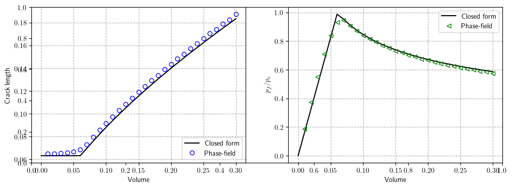
Under the toughness-dominated regime without leak-off, the fluid viscosity dissipation is negligible compared to the energy released for fracture surface formation (Detournay et al., 2016). Therefore, in this regime, we can neglect the pressure loss within the fracture and use the Sneddon solution for crack opening (Bourdin et al., 2012, Sneddon et al., 1969) to determine the pressure and length evolution.
The work of the pressure force is as follows:
$$ \begin{equation} \mathcal{W}(R) =\frac{2 p^2 a^2}{E'}. \end{equation} $$Applying Clapeyron’s theorem, the elastic energy can be determined as
$$ \begin{equation} \mathcal{E}(R) =-\frac{\pi p^2 a^2}{E'}, \end{equation} $$and the energy release rate with respect to the crack length $a$ propagating along the initial inclination is
$$ \begin{equation} G(R) = - \frac{\partial \mathcal{E}}{\partial (2 a)} = \frac{\pi p^2 a}{E'}. \end{equation} $$Griffith's criterion (Griffith et al., 1920) states that the fracture propagates when $G=G_c$ and the critical volume for crack propagation is $V_c := \sqrt{\dfrac{4 \pi G_c a^3}{E' }}$ in a quasi-static volume control setting (the fracture propagation is always unstable with pressure control).
The evolution of the corresponding pressure and fracture length
$$ \begin{equation} p(V) = \begin{cases} \dfrac{E' V}{2 \pi a_0^2} &\text{for} V < V_c \\ \left[ \dfrac{2 E' G_c^2}{\pi V} \right] ^{\frac{1}{3}}&\text{for} V \geq V_c, \end{cases} \end{equation} $$$$ \begin{equation} a(V) = \begin{cases} a_0 & V < V_c \\ \left[ \dfrac{E' V^2}{4 \pi G_c} \right ] ^{\frac{1}{3}} & V \geq V_c. \end{cases} \end{equation} $$Problem Description
Based on Sneddon's solution (Sneddon et al., 1969), we verified the model with plane-strain hydraulic fracture propagation in a toughness-dominated regime. In an infinite 2D domain, the problem was solved with a line fracture $[-a_0, a_0] \times \{0\}$ ($a_0$ = 0.05). We considered a large finite domain $[-40a_0,40a_0] \times [-40a_0,40a_0]$ to account for the infinite boundaries in the closed-form solution. The effective size of an element, $h$, is $1\times10^{-2}$.

- In order to have the hydraulic fracturing in the toughness dominated-regime, add, $\texttt{
propagating }$ in the project file. - Yoshioka et al., 2019 provides additional information on the implementation, use of real material properties, and rescaling of the phase-field energy functional.
Input Data
Taking advantage of the linearity of the system, the simulations were run with the dimensionless properties listed in the Table below.
| Name | Value | Symbol |
|---|---|---|
| Young’s modulus | 1 | $E$ |
| Poisson’s ratio | 0.15 | $\nu$ |
| Fracture toughness | 1 | $G_{c}$ |
| Regularization parameter | 2$h$ | $\ell_s$ |
| Length | 4 | $L$ |
| Height | 4 | $H$ |
| Initial crack length | 0.1 | $2a_0$ |
import math…
(click to toggle)
import math
import os
import re
import time
from pathlib import Path
from subprocess import run

import gmsh
import matplotlib.pyplot as plt
import numpy as np
import ogstools as ot
import pyvista as pvpi = math.pi
plt.rcParams["text.usetex"] = True
E = 1.0…
(click to toggle)
E = 1.0
nu = 0.15
Gc = 1.0
h = 0.01
a0 = 0.05  # half of the initial crack length

phasefield_model = "AT1" # AT1/AT2Output Directory and Project File
# file's name…
(click to toggle)
# file's name
prj_name = "Kregime_Propagating.prj"
meshname = "mesh_full_pf"

out_dir = Path(os.environ.get("OGS_TESTRUNNER_OUT_DIR", "_out"))
out_dir.mkdir(parents=True, exist_ok=True)Mesh Generation
def mesh_generation(lc, lc_fine):…
(click to toggle)
def mesh_generation(lc, lc_fine):
    """
    lc ... characteristic length for coarse meshing
    lc_fine ... characteristic length for fine meshing
    """
    L = 4.0  # Length
    H = 4.0  # Height
    b = 0.4  # Length/Height of subdomain with fine mesh

    # Before using any functions in the Python API, Gmsh must be initialized
    gmsh.initialize()
    gmsh.option.setNumber("General.Terminal", 1)
    gmsh.model.add("rectangle")

    # Dimensions
    dim0 = 0
    dim1 = 1
    dim2 = 2

    # Points
    gmsh.model.geo.addPoint(-L / 2, -H / 2, 0, lc, 1)
    gmsh.model.geo.addPoint(L / 2, -H / 2, 0, lc, 2)
    gmsh.model.geo.addPoint(L / 2, H / 2, 0, lc, 3)
    gmsh.model.geo.addPoint(-L / 2, H / 2, 0, lc, 4)
    gmsh.model.geo.addPoint(-b, -b - lc_fine / 2, 0, lc_fine, 5)
    gmsh.model.geo.addPoint(b, -b - lc_fine / 2, 0, lc_fine, 6)
    gmsh.model.geo.addPoint(b, b + lc_fine / 2, 0, lc_fine, 7)
    gmsh.model.geo.addPoint(-b, b + lc_fine / 2, 0, lc_fine, 8)

    # Lines
    gmsh.model.geo.addLine(1, 2, 1)
    gmsh.model.geo.addLine(2, 3, 2)
    gmsh.model.geo.addLine(3, 4, 3)
    gmsh.model.geo.addLine(4, 1, 4)
    gmsh.model.geo.addLine(5, 6, 5)
    gmsh.model.geo.addLine(6, 7, 6)
    gmsh.model.geo.addLine(7, 8, 7)
    gmsh.model.geo.addLine(8, 5, 8)

    # Line loops
    gmsh.model.geo.addCurveLoop([1, 2, 3, 4], 1)
    gmsh.model.geo.addCurveLoop([5, 6, 7, 8], 2)

    # Add plane surfaces defined by one or more curve loops.
    gmsh.model.geo.addPlaneSurface([1, 2], 1)
    gmsh.model.geo.addPlaneSurface([2], 2)

    gmsh.model.geo.synchronize()

    # Prepare structured grid
    gmsh.model.geo.mesh.setTransfiniteCurve(
        6, math.ceil(2 * b / lc_fine + 2), "Progression", 1
    )
    gmsh.model.geo.mesh.setTransfiniteCurve(
        8, math.ceil(2 * b / lc_fine + 2), "Progression", 1
    )
    gmsh.model.geo.mesh.setTransfiniteSurface(2, "Alternate")

    gmsh.model.geo.mesh.setRecombine(dim2, 1)
    gmsh.model.geo.mesh.setRecombine(dim2, 2)

    gmsh.model.geo.synchronize()

    # Physical groups
    P1 = gmsh.model.addPhysicalGroup(dim0, [1])
    gmsh.model.setPhysicalName(dim0, P1, "P1")

    P2 = gmsh.model.addPhysicalGroup(dim0, [2])
    gmsh.model.setPhysicalName(dim0, P2, "P2")

    Bottom = gmsh.model.addPhysicalGroup(dim1, [1])
    gmsh.model.setPhysicalName(dim1, Bottom, "Bottom")

    Right = gmsh.model.addPhysicalGroup(dim1, [2])
    gmsh.model.setPhysicalName(dim1, Right, "Right")

    Top = gmsh.model.addPhysicalGroup(dim1, [3])
    gmsh.model.setPhysicalName(dim1, Top, "Top")

    Left = gmsh.model.addPhysicalGroup(dim1, [4])
    gmsh.model.setPhysicalName(dim1, Left, "Left")

    Computational_domain = gmsh.model.addPhysicalGroup(dim2, [1, 2])
    gmsh.model.setPhysicalName(dim2, Computational_domain, "Computational_domain")
    gmsh.model.geo.synchronize()

    output_file = f"{out_dir}/" + meshname + ".msh"
    gmsh.model.mesh.generate(dim2)
    gmsh.write(output_file)
gmsh.finalize()Pre-Processing
def pre_processing(h, a0):…
(click to toggle)
def pre_processing(h, a0):
    mesh = pv.read(f"{out_dir}/mesh_full_pf_domain.vtu")
    phase_field = np.ones((len(mesh.points), 1))
    pv.set_plot_theme("document")

    for node_id, x in enumerate(mesh.points):
        if (
            (mesh.center[0] - x[0]) <= a0 + 0.001 * h
            and (mesh.center[0] - x[0]) >= -a0 - 0.001 * h
            and (mesh.center[1] - x[1]) < h / 2 + 0.001 * h
            and (mesh.center[1] - x[1]) > -h / 2 - 0.001 * h
        ):
            phase_field[node_id] = 0.0

    mesh.point_data["phase-field"] = phase_field
mesh.save(f"{out_dir}/mesh_full_pf_OGS_pf_ic.vtu")Run the Simulation
pv.set_plot_theme("document")…
(click to toggle)
pv.set_plot_theme("document")
pv.set_jupyter_backend("static")


def Hydraulic_Fracturing_Toughness_Dominated_numerical(h, phasefield_model):
    # mesh properties
    ls = 2 * h
    # generate prefix from properties
    filename = f"results_h_{h:0.4f}_{phasefield_model}"
    mesh_generation(0.1, h)
    # Convert GMSH (.msh) meshes to VTU meshes appropriate for OGS simulation.
    input_file = f"{out_dir}/" + meshname + ".msh"
    meshes = ot.meshes_from_gmsh(filename=input_file, log=False)
    for name, mesh in meshes.items():
        pv.save_meshio(f"{out_dir}/mesh_full_pf_{name}.vtu", mesh)
    %cd {out_dir}
    run(
        "identifySubdomains -f -m mesh_full_pf_domain.vtu -- mesh_full_pf_physical_group_*.vtu",
        shell=True,
        check=True,
    )
    %cd -

    # As a preprocessing step, define the initial phase-field (crack).
    pre_processing(h, a0)
    # change properties in prj file #For more information visit: https://ogstools.opengeosys.org/stable/reference/ogstools.ogs6py.html
    model = ot.Project(
        input_file=prj_name,
        output_file=f"{out_dir}/{prj_name}",
        MKL=True,
        args=f"-o {out_dir}",
    )
    model.replace_parameter_value(name="ls", value=ls)
    model.replace_text(phasefield_model, xpath="./processes/process/phasefield_model")
    model.replace_text(filename, xpath="./time_loop/output/prefix")
    model.write_input()
    # run simulation with ogs
    t0 = time.time()
    print(">>> OGS started execution ... <<<")
    run(
        f"ogs {out_dir}/{prj_name} -o {out_dir} > {out_dir}/log.txt",
        shell=True,
        check=True,
    )
    tf = time.time()
print(">>> OGS terminated execution <<< Elapsed time: ", round(tf - t0, 2), " s.")Hydraulic_Fracturing_Toughness_Dominated_numerical(h, phasefield_model)Info : Meshing 1D...
Info : [ 0%] Meshing curve 1 (Line)
Info : [ 20%] Meshing curve 2 (Line)
Info : [ 30%] Meshing curve 3 (Line)
Info : [ 40%] Meshing curve 4 (Line)
Info : [ 60%] Meshing curve 5 (Line)
Info : [ 70%] Meshing curve 6 (Line)
Info : [ 80%] Meshing curve 7 (Line)
Info : [ 90%] Meshing curve 8 (Line)
Info : Done meshing 1D (Wall 0.000459656s, CPU 0s)
Info : Meshing 2D...
Info : [ 0%] Meshing surface 1 (Plane, Frontal-Delaunay)
Info : [ 0%] Blossom: 24032 internal 482 closed
Info    : [  0%] Blossom recombination completed (Wall 0.732655s, CPU 0.34262s): 7878 quads, 0 triangles, 0 invalid quads, 0 quads with Q < 0.1, avg Q = 0.793024, min Q = 0.371315
Info    : [ 60%] Meshing surface 2 (Transfinite)
Info    : Done meshing 2D (Wall 1.11612s, CPU 0.496835s)
Info    : 14439 nodes 14848 elements
Info    : Writing '/var/lib/gitlab-runner/builds/vZ6vnZiU/0/ogs/build/release-petsc/Tests/Data/PhaseField/Kregime_Propagating_jupyter_notebook/Kregime_Propagating_jupyter/mesh_full_pf.msh'...
Info    : Done writing '/var/lib/gitlab-runner/builds/vZ6vnZiU/0/ogs/build/release-petsc/Tests/Data/PhaseField/Kregime_Propagating_jupyter_notebook/Kregime_Propagating_jupyter/mesh_full_pf.msh'
/var/lib/gitlab-runner/builds/vZ6vnZiU/0/ogs/build/release-petsc/Tests/Data/PhaseField/Kregime_Propagating_jupyter_notebook/Kregime_Propagating_jupyter
[0] info: Mesh reading time: 0.0827256 s
[0] info: MeshNodeSearcher construction time: 0.000509858 s
[0] info: identifySubdomainMesh(): identifySubdomainMeshNodes took 1.0981e-05 s
[0] info: There is already a 'bulk_node_ids' property present in the subdomain mesh 'mesh_full_pf_physical_group_Bottom' and it is equal to the newly computed values.
[0] info: identifySubdomainMesh(): identifySubdomainMeshElements took 0.00785734 s
[0] info: identifySubdomainMesh(): identifySubdomainMeshNodes took 0.00109892 s
[0] info: There is already a 'bulk_node_ids' property present in the subdomain mesh 'mesh_full_pf_physical_group_Computational_domain' and it is equal to the newly computed values.
[0] info: identifySubdomainMesh(): identifySubdomainMeshElements took 0.0147933 s
[0] info: identifySubdomainMesh(): identifySubdomainMeshNodes took 4.26e-06 s
[0] info: There is already a 'bulk_node_ids' property present in the subdomain mesh 'mesh_full_pf_physical_group_Left' and it is equal to the newly computed values.
[0] info: identifySubdomainMesh(): identifySubdomainMeshElements took 0.00058183 s
[0] info: identifySubdomainMesh(): identifySubdomainMeshNodes took 5.6e-07 s
[0] info: There is already a 'bulk_node_ids' property present in the subdomain mesh 'mesh_full_pf_physical_group_P1' and it is equal to the newly computed values.
[0] info: identifySubdomainMesh(): identifySubdomainMeshElements took 0.00056512 s
[0] info: identifySubdomainMesh(): identifySubdomainMeshNodes took 2.9e-07 s
[0] info: There is already a 'bulk_node_ids' property present in the subdomain mesh 'mesh_full_pf_physical_group_P2' and it is equal to the newly computed values.
[0] info: identifySubdomainMesh(): identifySubdomainMeshElements took 0.0005677 s
[0] info: identifySubdomainMesh(): identifySubdomainMeshNodes took 5.12e-06 s
[0] info: There is already a 'bulk_node_ids' property present in the subdomain mesh 'mesh_full_pf_physical_group_Right' and it is equal to the newly computed values.
[0] info: identifySubdomainMesh(): identifySubdomainMeshElements took 0.00055169 s
[0] info: identifySubdomainMesh(): identifySubdomainMeshNodes took 4.71e-06 s
[0] info: There is already a 'bulk_node_ids' property present in the subdomain mesh 'mesh_full_pf_physical_group_Top' and it is equal to the newly computed values.
[0] info: identifySubdomainMesh(): identifySubdomainMeshElements took 0.00656588 s
[0] info: identifySubdomains time: 0.0398408 s
[0] info: writing time: 0.0710347 s
[0] info: Entire run time: -8.98848e+06 s
/var/lib/gitlab-runner/builds/vZ6vnZiU/0/ogs/ogs/Tests/Data/PhaseField/Kregime_Propagating_jupyter_notebook
>>> OGS started execution ... <<<
>>> OGS terminated execution <<< Elapsed time: 815.56 s.
Post-Processing
Analytical Solution for the Evolution of Fracture Length and Pressure
def Analytical_solution(phasefield_model, h):…
(click to toggle)
def Analytical_solution(phasefield_model, h):
    v = np.linspace(1e-10, 0.3, 31)
    pres = np.linspace(0, 1.0, 31)
    length = np.linspace(0, 1.0, 31)

    ls = 2 * h

    # Effective Gc and a for AT1/A2
    if phasefield_model == "AT1":
        Gc_ref = Gc * (3 * h / 8.0 / ls + 1.0)
        a_eff = a0 * (1 + pi * ls / (4.0 * a0 * (3 * h / 8.0 / ls + 1.0)))
    elif phasefield_model == "AT2":
        Gc_ref = Gc * (h / (2.0 * ls) + 1.0)
        a_eff = a0 * (1 + pi * ls / (4.0 * a0 * (h / (2.0 * ls) + 1.0)))

    Eprime = E / (1 - nu**2)

    V_c = (4 * pi * Gc_ref * a_eff**3 / Eprime) ** 0.5
    P_c = (Eprime * Gc_ref / (pi * a_eff)) ** 0.5

    for i in range(len(v)):
        if v[i] < V_c:
            pres[i] = Eprime * v[i] / (2 * pi * a_eff**2) / P_c
            length[i] = a_eff
        else:
            pres[i] = (2 * Eprime * Gc_ref**2 / (pi * v[i])) ** 0.333333 / P_c
            length[i] = (Eprime * v[i] ** 2 / (4 * pi * Gc_ref)) ** 0.333333

    return v, pres, length, Gc_ref, P_c


fluidVolume_analytical = Analytical_solution(phasefield_model, h)[0]
pressure_analytical = Analytical_solution(phasefield_model, h)[1]
length_analytical = Analytical_solution(phasefield_model, h)[2]
Gc_ref = Analytical_solution(phasefield_model, h)[3]
P_c = Analytical_solution(phasefield_model, h)[4]Phase Field Versus Analytical Solution for Fracture Length and Pressure Evolution
In phase field approach, we can retrieve the crack length $a$ as:
$$ \begin{equation} a = \dfrac{\displaystyle \int_\Omega \frac{G_c}{4 c_n} \left(\frac{(1-v)^n}{\ell}+ \ell |\nabla v|^2\right)\,\mathrm{d} \Omega }{G_c \left( \dfrac{h}{4 c_n \ell} + 1 \right)}. \end{equation} $$where $n=1$ corresponds to $\texttt{AT}_1$ ($c_n = 2/3$) and $n=2$ to $\texttt{AT}_2$ ($c_n = 1/2$).
plt.subplots(figsize=(12, 4))…
(click to toggle)
plt.subplots(figsize=(12, 4))
plt.subplot(1, 2, 1)
fluid_volume = []
surface_energy = []
# Open the file for reading
with (out_dir / "log.txt").open() as fd:
    # Iterate over the lines
    for _i, line in enumerate(fd):
        match_surface_energy = re.search(
            r"""Surface energy: (\d+\.\d*) Pressure work: (\d+\.\d*)  at time: (\d+\.\d*)""",
            line,
        )
        if match_surface_energy:
            surface_energy.append(float(match_surface_energy.group(1)))
            fluid_volume.append(float(match_surface_energy.group(3)))

plt.grid(linestyle="dashed")
plt.xlabel("Volume")
plt.ylabel("Crack length")
plt.plot(fluidVolume_analytical, length_analytical, "black", label="Closed form")
plt.plot(
    fluid_volume,
    np.array(surface_energy[:]) / Gc_ref / 2,
    "bo",
    fillstyle="none",
    label="Phase-field",
)
legend = plt.legend(loc="lower right")

plt.subplot(1, 2, 2)
fluid_volume = []
pressure = []
# Open the file for reading
with (out_dir / "log.txt").open() as fd:
    # Iterate over the lines
    for _i, line in enumerate(fd):
        match_pressure = re.search(
            r"""Pressure: (\d+\.\d*) at time: (\d+\.\d*)""", line
        )
        if match_pressure:
            fluid_volume.append(float(match_pressure.group(2)))
            pressure.append(float(match_pressure.group(1)))


plt.xlabel("Volume")
plt.ylabel("$p_f/p_c$")
plt.plot(fluidVolume_analytical, pressure_analytical, "black", label="Closed form")
plt.plot(
    np.array(fluid_volume[:]),
    np.array(pressure[:]) / P_c,
    "g<",
    fillstyle="none",
    label="Phase-field",
)
plt.grid(linestyle="dashed")
legend = plt.legend(loc="upper right")
plt.show()
plt.subplots(figsize=(12, 4))…
(click to toggle)
plt.subplots(figsize=(12, 4))
plt.subplot(1, 2, 1)
plt.grid(linestyle="dashed")
plt.plot(
    fluidVolume_analytical[1:],
    (
        abs(length_analytical[1:] - np.array(surface_energy[:]) / (2 * Gc_ref))
        / (np.array(surface_energy[:]) / (2 * Gc_ref))
    )
    * 100,
    "-.ob",
    fillstyle="none",
    label="Closed form",
)
plt.ylim([0.0, 10])
plt.xlabel("Volume")
plt.ylabel(
    r"$\frac{|a_\mathrm{num}-{a}_\mathrm{ana}|}{{a}_\mathrm{num}}\times 100\%$",
    fontsize=14,
)

plt.subplot(1, 2, 2)
plt.grid(linestyle="dashed")
plt.plot(
    fluidVolume_analytical[1:],
    (abs(pressure_analytical[1:] - np.array(pressure[:]) / P_c) / pressure[:]) * 100,
    "-.<g",
    fillstyle="none",
    label="Closed form",
)
plt.ylim([0.0, 10])
plt.xlabel("Volume")
plt.ylabel(
    r"$\frac{|p_\mathrm{num}-{p}_\mathrm{ana}|}{{p}_\mathrm{num}}\times 100\%$",
    fontsize=14,
)
plt.show()
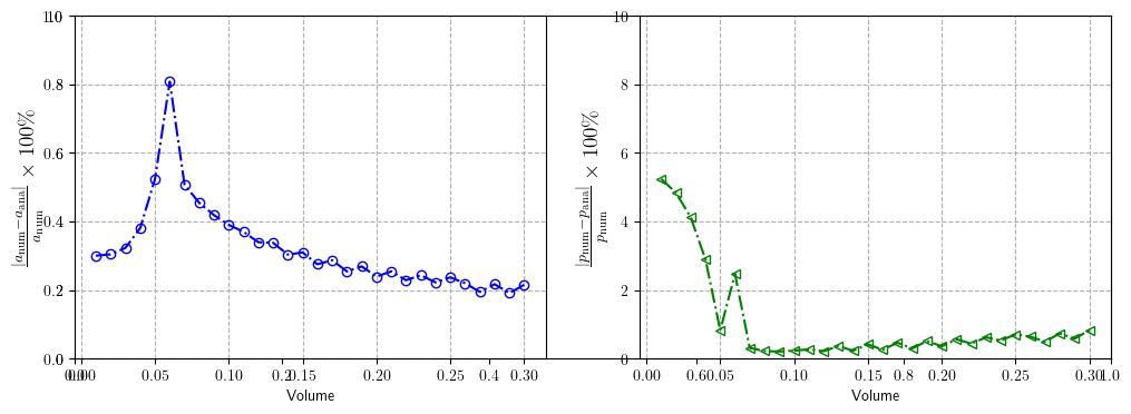
In order to reduce computation time, we perform the simulation with a coarse mesh; the results for the $\texttt{AT}_1$ Model with a mesh size of $h=0.001$ are provided below.
$\texttt{AT}_1$ Model:


Hydraulic Fracturing Animation (Using Phase Field Approach)
filename = f"results_h_{h:0.4f}_{phasefield_model}"…
(click to toggle)
filename = f"results_h_{h:0.4f}_{phasefield_model}"
reader = pv.get_reader(f"{out_dir}/" + filename + ".pvd")

plotter = pv.Plotter(shape=(1, 2), border=False)
plotter.open_gif(f"{out_dir}/Kregime_Propagating.gif")
for time_value in reader.time_values:
    reader.set_active_time_value(time_value)
    mesh = reader.read()[0]
    sargs = {
        "title": "Phase field",
        "title_font_size": 16,
        "label_font_size": 12,
        "n_labels": 5,
        "position_x": 0.25,
        "position_y": 0.15,
        "fmt": "%.1f",
        "width": 0.5,
    }
    p = pv.Plotter(shape=(1, 2), border=False)
    clim = [0, 1.0]
    points = mesh.point_data["phasefield"].shape[0]
    xs = mesh.points[:, 0]
    ys = mesh.points[:, 1]
    pf = mesh.point_data["phasefield"]
    plotter.clear()
    plotter.add_mesh(
        mesh,
        scalars=pf,
        show_scalar_bar=True,
        colormap="coolwarm",
        clim=clim,
        scalar_bar_args=sargs,
        lighting=False,
    )
    plotter.add_text(f"Time: {time_value:0.02f}", color="black")

    plotter.view_xy()
    plotter.write_frame()

plotter.close()[0m[33m2026-01-30 13:19:03.790 ( 835.880s) [ 7F6BAC047BC0]vtkXOpenGLRenderWindow.:1416 WARN| bad X server connection. DISPLAY=[0m
Phase Field Profile at Last Time Step
mesh = reader.read()[0]…
(click to toggle)
mesh = reader.read()[0]

points = mesh.point_data["phasefield"].shape[0]
xs = mesh.points[:, 0]
ys = mesh.points[:, 1]
pf = mesh.point_data["phasefield"]

clim = [0, 1.0]
sargs = {
    "title": "Phase field",
    "title_font_size": 16,
    "label_font_size": 12,
    "n_labels": 5,
    "position_x": 0.25,
    "position_y": 0.0,
    "fmt": "%.1f",
    "width": 0.5,
}
plotter = pv.Plotter(shape=(1, 2), border=False)
plotter.add_mesh(
    mesh,
    scalars=pf,
    show_edges=False,
    show_scalar_bar=True,
    colormap="coolwarm",
    clim=clim,
    scalar_bar_args=sargs,
    lighting=False,
)

plotter.view_xy()
plotter.camera.zoom(1.5)
plotter.window_size = [1000, 500]
plotter.show()Widget(value='<iframe src="http://localhost:46085/index.html?ui=P_0x7f6b62f8f750_31&reconnect=auto" class="pyv…
References
[1] Detournay, Emmanuel. Mechanics of hydraulic fractures. Annual review of fluid mechanics 48 (2016): 311-339.
[2] Bourdin, Blaise, Chukwudi Chukwudozie, and Keita Yoshioka. A variational approach to the numerical simulation of hydraulic fracturing. In SPE annual technical conference and exhibition. OnePetro, 2012.
[3] Sneddon, Ian Naismith, and Morton Lowengrub. Crack problems in the classical theory of elasticity. 1969, 221 P (1969).
[4] Griffith, Alan Arnold. VI. The phenomena of rupture and flow in solids. Philosophical transactions of the royal society of london. Series A, containing papers of a mathematical or physical character 221, no. 582-593 (1921): 163-198.
[5] Yoshioka, Keita, Francesco Parisio, Dmitri Naumov, Renchao Lu, Olaf Kolditz, and Thomas Nagel. Comparative verification of discrete and smeared numerical approaches for the simulation of hydraulic fracturing. GEM-International Journal on Geomathematics 10, no. 1 (2019): 1-35.
This article was written by Mostafa Mollaali, Keita Yoshioka. If you are missing something or you find an error please let us know.
Generated with Hugo 0.147.9
in CI job 683680
|
Last revision: March 3, 2023