Volumetric Source Term

Elliptic/square_1x1_SteadyStateDiffusion/square_1e2_volumetricsourceterm.prj

Equations

We start with Poisson equation:

$$ \begin{equation} \- k\\; \Delta p = Q \quad \text{in }\Omega \end{equation}$$

w.r.t boundary conditions

$$ \eqalign{ p(x) = g_D(x) &\quad \text{on }\Gamma_D,\cr k\\;{\partial p(x) \over \partial n} = g_N(x) &\quad \text{on }\Gamma_N, }$$

where $p$ could be the pressure, the subscripts $D$ and $N$ denote the Dirichlet- and Neumann-type boundary conditions, $n$ is the normal vector pointing outside of $\Omega$, and $\Gamma = \Gamma_D \cup \Gamma_N$ and $\Gamma_D \cap \Gamma_N = \emptyset$.

Problem specification and analytical solution

We solve the Poisson equation on a square domain $[0\times 1]^2$ with $k = 1$ w.r.t. the specific boundary conditions:

$$ \eqalign{ p(x,y) = 1 &\quad \text{on } (x=0,y) \subset \Gamma_D,\cr p(x,y) = 0 &\quad \text{on } (x=1,y) \subset \Gamma_D,\cr k\\;{\partial p(x,y) \over \partial n} = 0 &\quad \text{on }\Gamma_N. }$$

and the source term is $Q=1$.

The solution of this problem is

$$ p(x,y) = - \frac{1}{2} (x^2 + x) + 1. $$

Input files

The main project file is square_1e2_volumetricsourceterm.prj. It describes the processes to be solved and the related process variables together with their initial and boundary conditions. It also references the bulk mesh and the boundary meshes associated with the bulk mesh.

Running simulation

To start the simulation (after successful compilation) run:

ogs square_1e2_volumetricsourceterm.prj

OGS writes the computed results (pressure, Darcy velocity) into the output file square_1e2_volumetricsourceterm_pcs_0_ts_1_t_1.000000.vtu, which can be directly visualized and analysed in ParaView for example.

The output on the console will be similar to:

info: ConstantParameter: K
info: ConstantParameter: p0
info: ConstantParameter: p_Dirichlet_left
info: ConstantParameter: p_Dirichlet_right
info: ConstantParameter: volumetric_source_term_parameter
info: Initialize processes.
info: Solve processes.
info: [time] Output of timestep 0 took 0.000145912 s.
info: === Time stepping at step #1 and time 1 with step size 1
info: [time] Assembly took 0.000147104 s.
info: [time] Applying Dirichlet BCs took 1.81198e-05 s.
info: ------------------------------------------------------------------
info: *** Eigen solver computation
info: -> solve with CG (precon DIAGONAL)
info:    iteration: 11/10000
info:    residual: 3.965614e-17

info: ------------------------------------------------------------------
info: [time] Linear solver took 7.79629e-05 s.
info: [time] Iteration #1 took 0.000268221 s.
info: [time] Solving process #0 took 0.000288963 s in time step #1
info: [time] Time step #1 took 0.000308037 s.
info: [time] Output of timestep 1 took 0.000105858 s.
info: The whole computation of the time stepping took 1 steps, in which
         the accepted steps are 1, and the rejected steps are 0.

info: [time] Execution took 0.00692892 s.
info: OGS terminated on 2018-10-12 06:30:13+020

Results and evaluation

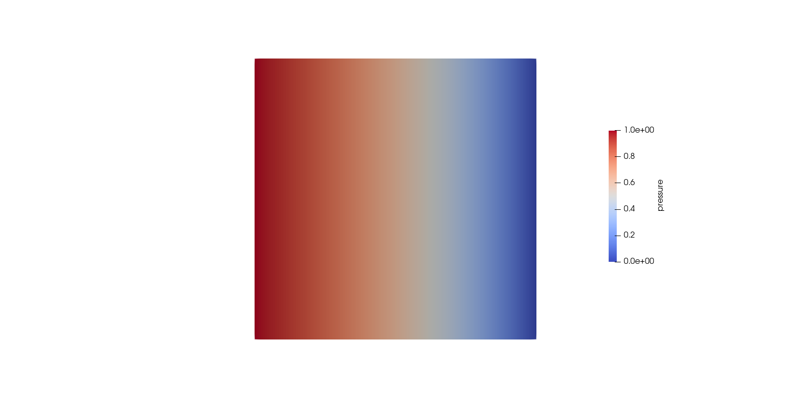
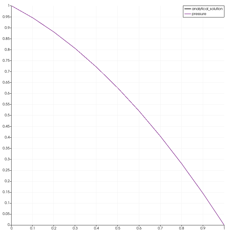
Comparison of the analytical solution and the computed solution

The numerical solution shown in the following picture is almost a linear gradient:

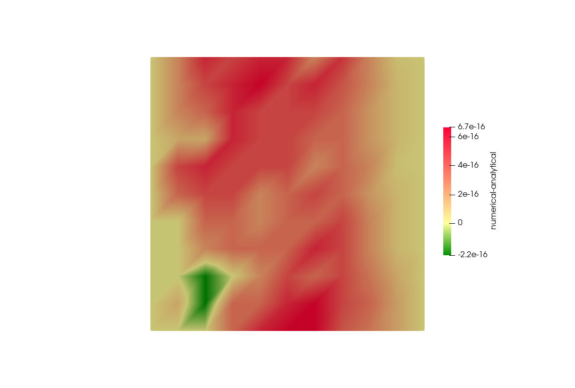
The line plot along the $x$ axis shows that the solution is a quadratic function and is in very good agreement to the analytical solution:

The difference between the computed solution and the analytical solution is in the range of machine precision and therefore almost negligible:

This article was written by Tom Fischer. If you are missing something or you find an error please let us know.
Generated with Hugo 0.122.0 in CI job 504124 | Last revision: November 12, 2024
Commit: [BL/MPI] Use MPI_COMM_WORLD in reduceMin 4aae83e | Edit this page on