Dirichlet-type boundary conditions

• Elliptic/square_1x1_SteadyStateDiffusion/square_1e2.xml

Equations

We start with simple linear homogeneous elliptic problem:

w.r.t boundary conditions

where $h$ could be hydraulic head, the subscripts $D$ and $N$ denote the Dirichlet- and Neumann-type boundary conditions, $n$ is the normal vector pointing outside of $\Omega$, and $\Gamma = \Gamma_D \cup \Gamma_N$ and $\Gamma_D \cap \Gamma_N = \emptyset$.

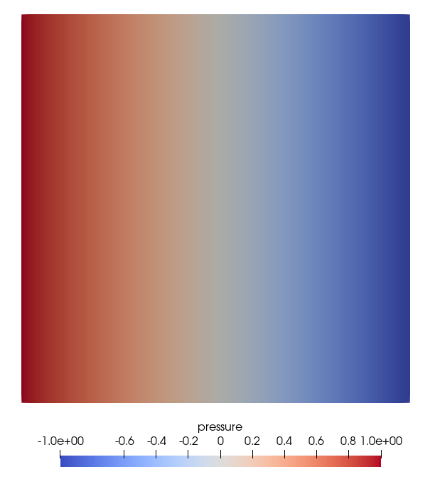
Problem specification and analytical solution

We solve the Laplace equation on a square domain $[0\times 1]^2$ with $k = 1$ w.r.t. the specific boundary conditions:

The solution of this problem is

Input files

The main project file is square_1e2.prj. It describes the processes to be solved and the related process variables together with their initial and boundary conditions. It also references the mesh and geometrical objects defined on the mesh.

As of now a small portion of possible inputs is implemented; one can change:

• the mesh file
• the geometry file
• introduce more/different Dirichlet boundary conditions (different geometry or values)

The geometries used to specify the boundary conditions are given in the square_1x1.gml file.

The input mesh square_1x1_quad_1e2.vtu is stored in the VTK file format and can be directly visualized in ParaView for example.

Running simulation

To start the simulation (after successful compilation) run:

ogs square_1e2.prj

It will produce the output files square_1e2_pcs_0.pvd, square_1e2_pcs_0_ts_0_t_0.000000.vtu and square_1e2_pcs_0_ts_1_t_1.000000.vtu. The last file contains the results computed in the first time step.

The output on the console will be similar to the following one (ignore the spurious error messages “Could not find POINT…”):

error: GEOObjects::getGeoObject(): Could not find POINT "left" in geometry.
error: GEOObjects::getGeoObject(): Could not find POINT "right" in geometry.
info: Initialize processes.
info: Solve processes.
info: -> max. absolute value of diagonal entries = 2.666667e-06
info: -> penalty scaling = 1.000000e+10
info: ------------------------------------------------------------------
info: *** LIS solver computation
info: -> solve
initial vector x      : user defined
precision             : double
linear solver         : CG
preconditioner        : none
convergence condition : ||b-Ax||_2 <= 1.0e-16 * ||b-Ax_0||_2
matrix storage format : CSR
linear solver status  : normal end

info:    iteration: 28/1000000

info:    residual: 3.004753e-17

info: ------------------------------------------------------------------

A major part of the output was produced by the linear equation solver (LIS in this case).

Results and evaluation