Neumann-type boundary conditions

Equations

We start with simple linear homogeneous elliptic problem:

w.r.t boundary conditions

where $h$ could be hydraulic head, the subscripts $D$ and $N$ denote the Dirichlet- and Neumann-type boundary conditions, $n$ is the normal vector pointing outside of $\Omega$, and $\Gamma = \Gamma_D \cup \Gamma_N$ and $\Gamma_D \cap \Gamma_N = \emptyset$.

Problem specification and analytical solution

We solve the Laplace equation on a square domain $[0\times 1]^2$ with $k = 1$ w.r.t. the specific boundary conditions:

The solution of this problem is

where

and

Input files

The main project file is square_1e2_neumann.prj. It describes the processes to be solved and the related process variables together with their initial and boundary conditions. It also references the mesh and geometrical objects defined on the mesh.

As of now a small portion of possible inputs is implemented; one can change:

• the mesh file
• the geometry file
• introduce more/different Dirichlet boundary conditions (different geometry or other constant values)
• introduce more/different Neumann boundary conditions (different geometry or other constant values)

The geometries used to specify the boundary conditions are given in the square_1x1.gml file.

The input mesh square_1x1_quad_1e2.vtu is stored in the VTK file format and can be directly visualized in ParaView for example.

Running simulation

To start the simulation (after successful compilation) run:

ogs square_1e2_neumann.prj

It will produce some output and write the computed result into the square_1e2_neumann.vtu for visualization with ParaView.

The output on the console will be similar to the following one (ignore the spurious error messages “Could not find POINT…”):

info: This is OpenGeoSys-6 version 6.0.7-619-ge761162.
info: OGS started on 2016-12-05 11:16:47+0100.
info: ConstantParameter: K
info: ConstantParameter: p0
info: ConstantParameter: p_neumann
info: ConstantParameter: p_Dirichlet
info: Lis options: "-initx_zeros 0 -i cg -p jacobi -tol 1e-16 -maxiter 10000"
info: Initialize processes.
info: Calculated search length for mesh "square_1x1_quad_1e2" is 1.000000e-09.
info: Solve processes.
info: [time] Output took 0.00378108 s.
info: === timestep #1 (t=1s, dt=1s) ==============================
info: [time] Assembly took 0.000336885 s.
info: [time] Applying Dirichlet BCs took 3.60012e-05 s.
info: ------------------------------------------------------------------
info: *** LIS solver computation
info: -> precon: 1
info: -> solver: 1
info: -> solve
info: -> status: 0
info: -> iteration: 35
info: -> residual: 6.16949e-17
info: -> time total           (s): 0.000153065
info: -> time iterations      (s): 0.000147343
info: -> time preconditioning (s): 5.72205e-06
info: -> time precond. create (s): 0
info: -> time precond. iter   (s): 5.72205e-06
info: ------------------------------------------------------------------
info: [time] Linear solver took 0.000437021 s.
info: [time] Iteration #1 took 0.000844002 s.
info: [time] Solving process #0 took 0.0011301 s in timestep #1.
info: [time] Output took 0.00462508 s.
info: [time] Timestep #1 took 0.00580406 s.
info: OGS terminated on 2016-12-05 11:16:47+010
info: [time] Execution took 0.016582 s.

A last major part of the output was produced by the linear equation solver (LIS in this case) showing good convergence.

Results and evaluation

Compared to the analytical solution presented above the results are very good but in a single point:

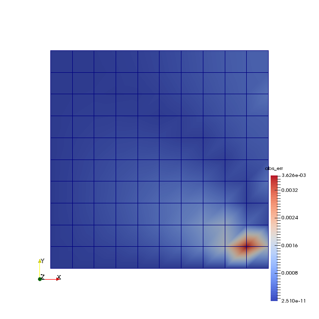
Both Dirichlet boundary conditions are satisfied. The values of gradients in x direction along the right side and y directions along the top sides of the domain a shown below:

The homogeneous Neumann boundary condition on the top side is satisfied (ScalarGradient_Y is close to zero). The inhomogeneous Neumann boundary condition on the bottom is satisfied only for $y > 0.3$ (where the ScalarGradient_X is close to one) because of incompatible boundary conditions imposed on the bottom right corner of the domain.