Simulating the Selke 2D process with Dirichlet and Neumann Boundary Constraints
 This page is based on a Jupyter notebook.



Simulating the Selke 2D process with Dirichlet and Neumann Boundary Constraints
The River Selke is a fourth-order stream with a length of 64 km draining a part of the forested Harz Mountains and the agriculturally dominated Northern Harz foreland in Central Germany. Due to different water management targets such as the design of infiltration wells along a former pit mine the area is of particular interest for hydrogeological research (cf. Nixdorf et al., 2025 ) In this notebook we show how to append the previous notebook on the Selke 2D process to include a source term and Neumann boundary condition for the upstream boundary
import numpy as np…
(click to toggle)
import numpy as np
import ogstools as ot
import pyvista as pv

ot.plot.setup.show_region_bounds = False1 Load data and run Dirichlet simulation
We begin by loading the necessary meshes and the original project file which we want to modify.
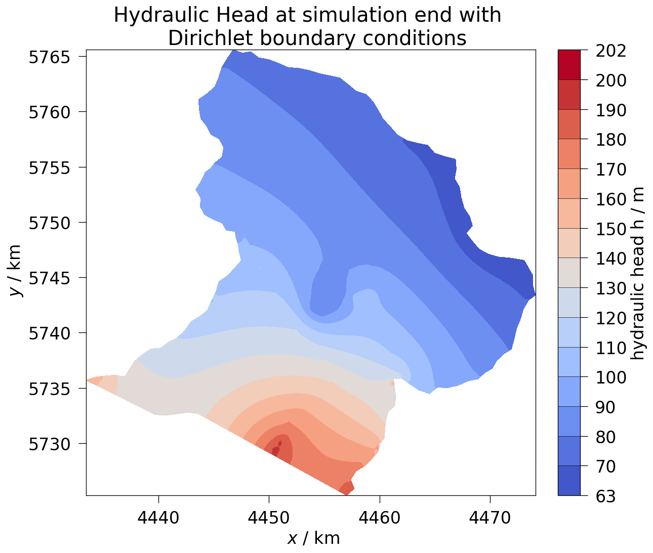
We also set up and run the original simulation with only Dirichlet boundary constraints so we can use it as a point of comparison later.
# Load Project-File…
(click to toggle)
# Load Project-File
project_dirichlet = ot.Project("Selke_Basin.prj").copy()
# Load Meshes
input_meshes = [
    "Selke_Basin_Domain_homo.vtu",
    "Selke_Basin_PG_Concordia.vtu",
    "Selke_Basin_PG_Koenigsauer.vtu",
    "Selke_Basin_PG_Wilsleber.vtu",
    "Selke_Basin_PL_Bode.vtu",
    "Selke_Basin_PL_Wipper.vtu",
    "Selke_Basin_Pnt_Wells.vtu",
    "Selke_Basin_PL_Selke.vtu",
    "Selke_Basin_PL_Upstream.vtu",
    "Selke_Basin_PG_recharge.vtu",
]
meshes = ot.Meshes.from_files(input_meshes)
output_names_dict = {
    "Selke_Basin_Domain_homo": "Selke Basin",
    "Selke_Basin_PG_Concordia": "Lake Concordia",
    "Selke_Basin_PG_Koenigsauer": "Lake Königsauer",
    "Selke_Basin_PG_Wilsleber": "Lake Wilsleber",
    "Selke_Basin_PL_Bode": "River Bode",
    "Selke_Basin_PL_Wipper": "River Wipper",
    "Selke_Basin_Pnt_Wells": "Wells",
    "Selke_Basin_PL_Selke": "River Selke",
    "Selke_Basin_PL_Upstream": "Upstream",
    "Selke_Basin_PG_recharge": "Selke Basin Recharge",
}
meshes.rename_output_names(output_names_dict)

# Set up and run Dirichlet simulation
model_dirichlet = ot.Model(project=project_dirichlet, meshes=meshes)
sim_dirichlet = model_dirichlet.run()
assert sim_dirichlet.status == ot.Simulation.Status.done

sim_dirichlet.meshseries.scale(spatial="km", time="d")
sim_dirichlet.meshseries.point_data["hydraulic head h / m"] = (
    sim_dirichlet.meshseries.point_data["pressure"] / (1000 * 9.81)
)
print(f"Simulation status: {sim_dirichlet.status_str}")
fig_dirichlet = ot.plot.contourf(
    sim_dirichlet.meshseries[-1], "hydraulic head h / m", fontsize=20
)
fig_dirichlet.axes[0].set_title(
    "Hydraulic Head at simulation end with \n  Dirichlet boundary conditions",
    fontsize=24,
    loc="center",
)Simulation status: Status: completed successfully (results available)
Text(0.5, 1.0, 'Hydraulic Head at simulation end with \n Dirichlet boundary conditions')
2 Modify the project file
We need to update the project file to accommodate the additional information we want to consider in the simulation.
This can be done manually with a text editor but OGSTools already incorporates bespoke functions which take care of the formal requirements of an OGS project file for us.
project_neumann = ot.Project("Selke_Basin.prj").copy()…
(click to toggle)
project_neumann = ot.Project("Selke_Basin.prj").copy()
project_neumann.mesh.add_mesh("Selke_Basin_PL_Upstream.vtu")
project_neumann.mesh.add_mesh("Selke_Basin_PG_recharge.vtu")2.1 Add a source term.
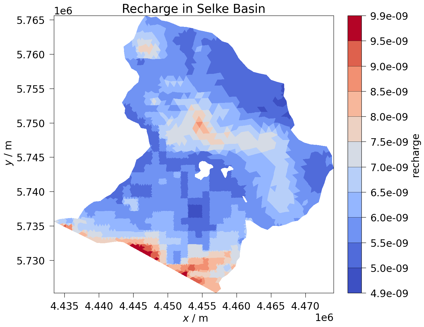
We first want to add a source term to the project file to specify the groundwater recharge rate of the region
project_neumann.parameters.add_parameter(…
(click to toggle)
project_neumann.parameters.add_parameter(
    name="q_recharge",
    type="MeshElement",
    mesh="Selke_Basin_PG_recharge",
    field_name="recharge",
)
project_neumann.process_variables.add_st(
    process_variable_name="pressure",
    type="Volumetric",
    mesh="Selke_Basin_PG_recharge",
    parameter="q_recharge",
)
# Visualise recharge
fig_recharge = ot.plot.contourf(
    meshes["Selke_Basin_PG_recharge"], "recharge", fontsize=20, lw=0.6
)
fig_recharge.axes[0].set_title(
    "Recharge in Selke Basin",
    fontsize=24,
    loc="center",
)Text(0.5, 1.0, 'Recharge in Selke Basin')
2.2 Add upstream boundary conditions
The upstream boundary is not chosen to conform to any hydrographic entity but in the transitional area of the Harz and the adjacent lowlands.
It is therefore unrealistic to assume a no-flow boundary condition (as we have implicitly done in the Dirichlet version of the Notebook).
Instead we want to describe the flow via Neumann boundary conditions.
Since we don’t have measurements we approximate the groundwater inflow as $0.1 \frac{m}{d}$ which implies a Darcy-Flux of $q_D=\phi v_f= 2.0*10^{-7}\frac{m}{s}$.
project_neumann.parameters.add_parameter( name=“q_upstream”, type=“Constant”, value=2.0e-7 ) project_neumann.process_variables.add_bc( process_variable_name=“pressure”, type=“Neumann”, mesh=“Selke_Basin_PL_Upstream”, parameter=“q_upstream”, )
# Optional: Save the modified project file
# project_neumann.save("Path of folder in which to save")3 Build the model and run the simulation
model_neumann = ot.Model(project=project_neumann, meshes=meshes)…
(click to toggle)
model_neumann = ot.Model(project=project_neumann, meshes=meshes)
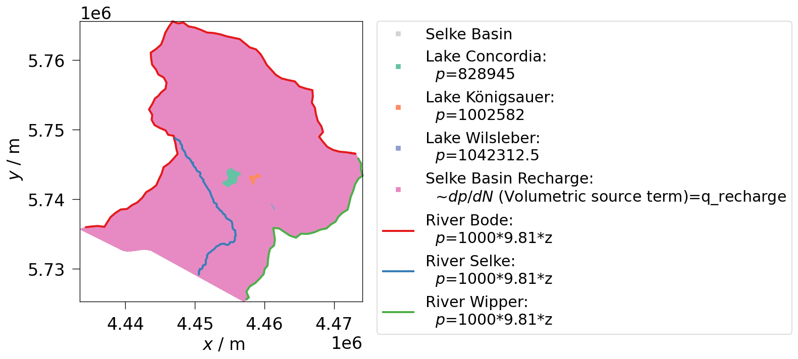
model_neumann.plot_constraints(fontsize=20, lw=0.6)
sim_neumann = model_neumann.run()
assert sim_neumann.status == ot.Simulation.Status.done
sim_neumann.meshseries.scale(spatial="km", time="d")
print(f"Simulation status: {sim_neumann.status_str}")Simulation status: Status: completed successfully (results available)
4 Analyse the result
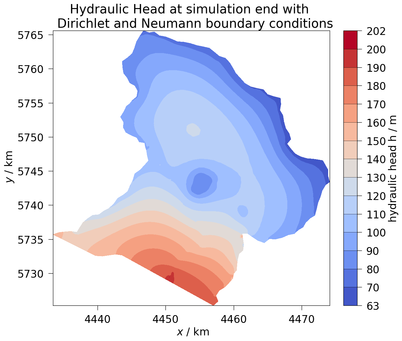
sim_neumann.meshseries.point_data["hydraulic head h / m"] = (…
(click to toggle)
sim_neumann.meshseries.point_data["hydraulic head h / m"] = (
    sim_neumann.meshseries.point_data["pressure"] / (1000 * 9.81)
)
fig_neumann = ot.plot.contourf(
    sim_neumann.meshseries[-1], "hydraulic head h / m", fontsize=20
)
fig_neumann.axes[0].set_title(
    "Hydraulic Head at simulation end with \n  Dirichlet and Neumann boundary conditions",
    fontsize=24,
    loc="center",
)
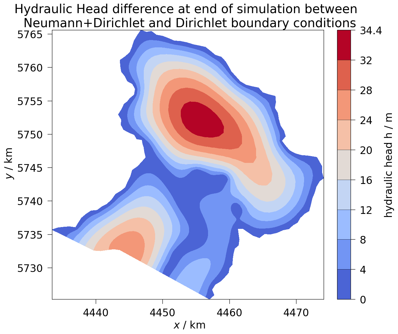
series_diff = ot.MeshSeries.difference(
    ms_a=sim_neumann.meshseries, ms_b=sim_dirichlet.meshseries
)
fig_difference = ot.plot.contourf(series_diff[-1], "hydraulic head h / m", fontsize=20)
fig_difference.axes[0].set_title(
    "Hydraulic Head difference at end of simulation between \n Neumann+Dirichlet and Dirichlet boundary conditions",
    fontsize=24,
    loc="center",
)Text(0.5, 1.0, 'Hydraulic Head difference at end of simulation between \n Neumann+Dirichlet and Dirichlet boundary conditions')
5 Depth to Groundwater
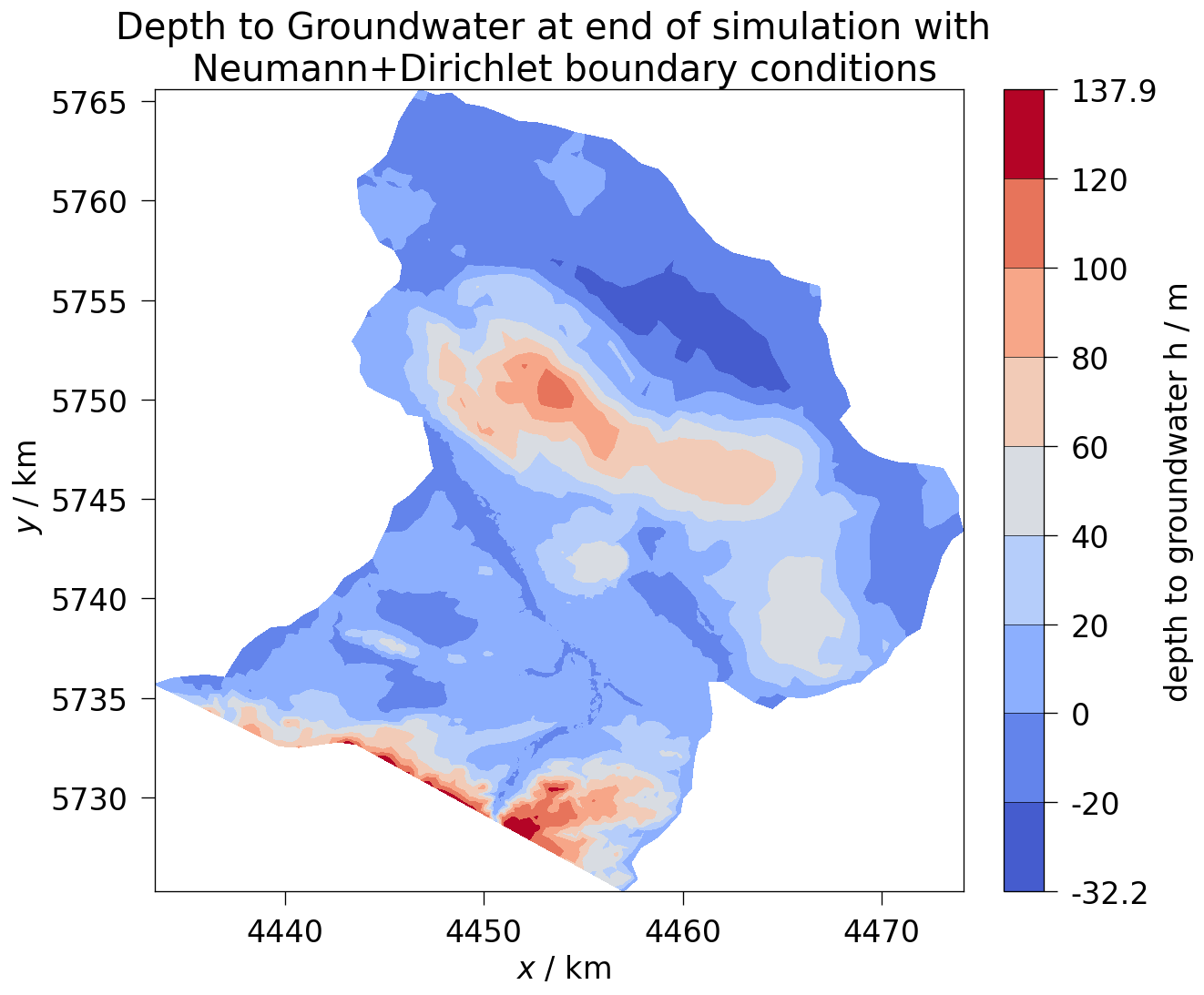
Finally, we can show depth to groundwater by subtracting hydraulic head from the z-coordinate at all mesh points
for mesh in sim_neumann.meshseries:…
(click to toggle)
for mesh in sim_neumann.meshseries:
    mesh.point_data["depth to groundwater h / m"] = (
        mesh.points[:, 2] * 1000 - mesh.point_data["hydraulic head h / m"]
    )
fig_depthgw = ot.plot.contourf(
    sim_neumann.meshseries[-1], "depth to groundwater h / m", fontsize=20
)
fig_depthgw.axes[0].set_title(
    "Depth to Groundwater at end of simulation with \n Neumann+Dirichlet boundary conditions",
    fontsize=24,
    loc="center",
)Text(0.5, 1.0, 'Depth to Groundwater at end of simulation with \n Neumann+Dirichlet boundary conditions')
# Check that simulations have produced expected outputs…
(click to toggle)
# Check that simulations have produced expected outputs
# The same test as at the end of the previous notebook. Since we had to run the Dirichlet simulation again for comparison we check its outputs again.
sim_dirichlet_expected = pv.read("expected_dirichlet.vtu")
np.testing.assert_allclose(
    sim_dirichlet.meshseries[-1]["pressure"],
    sim_dirichlet_expected["pressure"],
    atol=1e-10,
)
# Test of the new simulation. The tolerance is higher since the results can not be guaranteed to be as exact across devices as above.
sim_neumann_expected = pv.read("expected_neumann.vtu")
np.testing.assert_allclose(
    sim_neumann.meshseries[-1]["pressure"], sim_neumann_expected["pressure"], rtol=4e-3
)OGS links
- Project files:
- Original Project file: Selke_Basin.prj
- Mesh files:
References
- Nixdorf, E., Sips, M., & Morstein, P. (2025). Development of a digital workflow for layer reduction strategies and visual-analytical outcome analysis to enhance geo-hydraulic modelling efficiency. Digital Water, 3(1), 1-24. doi:10.1080/28375807.2025.2460825