Simulating the Selke 2D process with Dirichlet Boundary Constraints
 This page is based on a Jupyter notebook.



Simulating the Selke 2D process with Dirichlet Boundary Constraints
The River Selke is a fourth-order stream with a length of 64 km draining a part of the forested Harz Mountains and the agriculturally dominated
Northern Harz foreland in Central Germany. Due to different water management targets such as the design of infiltration wells along a former pit
mine the area is of particular interest for hydrogeological research (cf. Nixdorf et al., 2025
)
In this notebook we show how to build a OpenGeoSys model from given Project-Files and Mesh-Data, run it and analyse the results.
For this we use the ogstools Python-library, as shown in this workflow
.
The example used in this demonstration is a LiquidFLow process with Dirichlet boundary conditions of the Selke Basin.
import numpy as np…
(click to toggle)
import numpy as np
import ogstools as ot
import pyvista as pv
from matplotlib import pyplot as plt

ot.plot.setup.show_region_bounds = False1. Load data
Before we can build and run the model with ogstools we have to load a Project-File and Meshes which we have prepared or received beforehand.
To check that our Mesh-Data has been read correctly, we can plot the topology.
# Load Project-File…
(click to toggle)
# Load Project-File
project = ot.Project("Selke_Basin.prj")
# Load Meshes
input_meshes = [
    "Selke_Basin_Domain_homo.vtu",
    "Selke_Basin_PG_Concordia.vtu",
    "Selke_Basin_PG_Koenigsauer.vtu",
    "Selke_Basin_PG_Wilsleber.vtu",
    "Selke_Basin_PL_Bode.vtu",
    "Selke_Basin_PL_Wipper.vtu",
    "Selke_Basin_Pnt_Wells.vtu",
    "Selke_Basin_PL_Selke.vtu",
]
meshes = ot.Meshes.from_files(input_meshes)
output_names_dict = {
    "Selke_Basin_Domain_homo": "Selke Basin",
    "Selke_Basin_PG_Concordia": "Lake Concordia",
    "Selke_Basin_PG_Koenigsauer": "Lake Königsauer",
    "Selke_Basin_PG_Wilsleber": "Lake Wilsleber",
    "Selke_Basin_PL_Bode": "River Bode",
    "Selke_Basin_PL_Wipper": "River Wipper",
    "Selke_Basin_Pnt_Wells": "Wells",
    "Selke_Basin_PL_Selke": "River Selke",
}
meshes.rename_output_names(output_names_dict)1.1 Visualise Topology
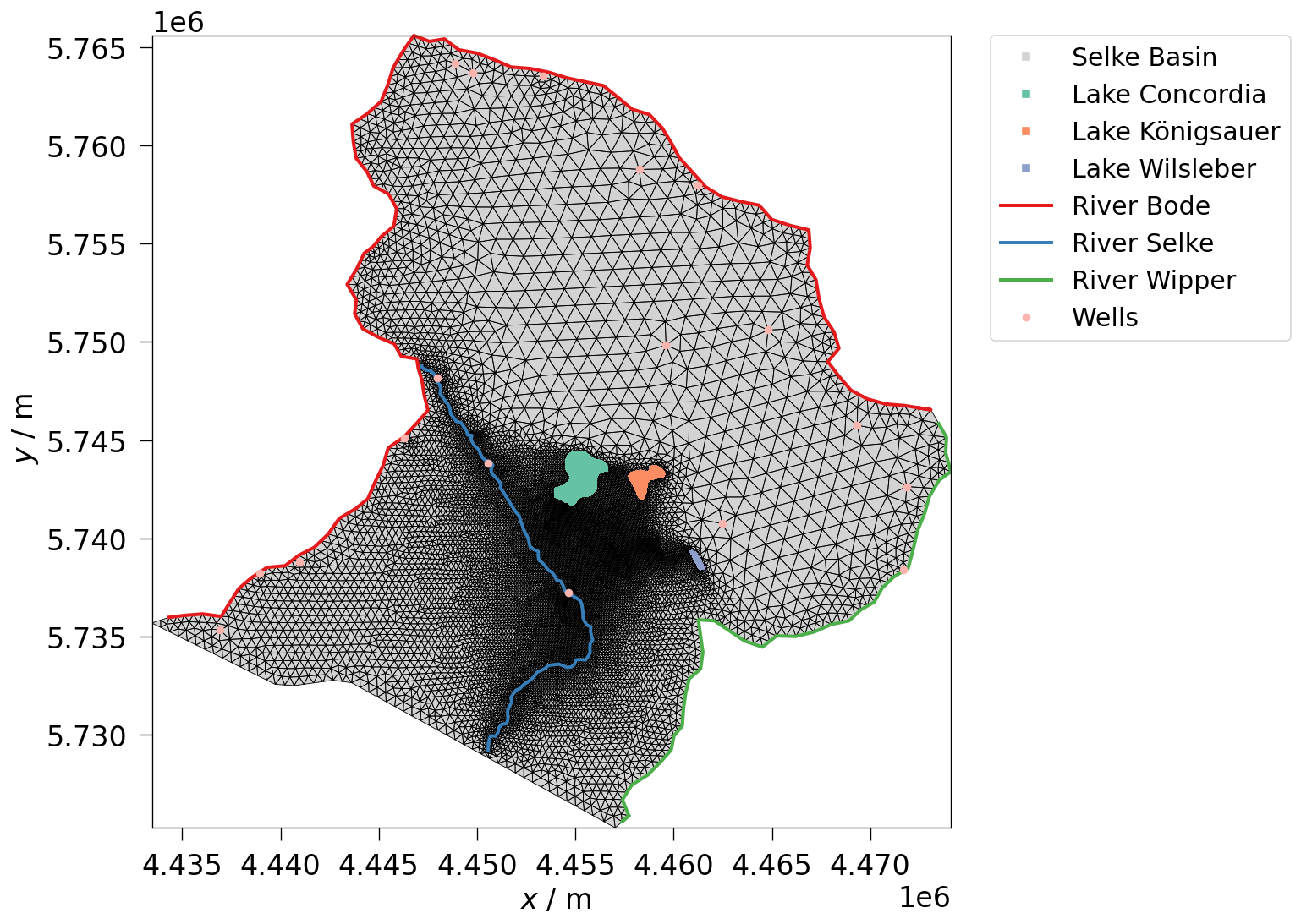
OGSTools includes a native functionality to visualise the domain mesh and all submeshes in one image.
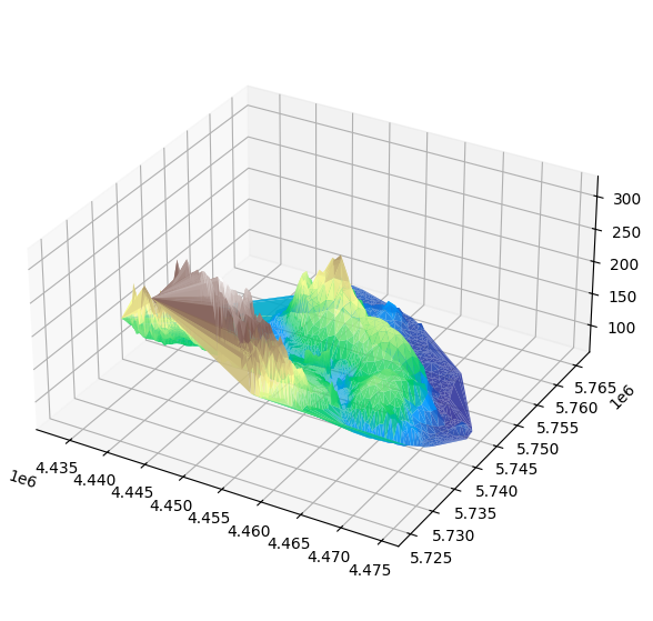
For simplicity, the geometry is projected onto the X-Y-surface. To see the height values included in the domain meshes we have to fall back on Matplotlib
# Visualise Meshes via OGSTools
fig_topology = meshes.plot(fontsize=20, lw=0.6)
# Visualise domain mesh in 3D with Matplotlib…
(click to toggle)
# Visualise domain mesh in 3D with Matplotlib
points = meshes.domain.points.copy()
fig = plt.figure(figsize=(10, 7))
ax = fig.add_subplot(111, projection="3d")
ax.plot_trisurf(
    points[:, 0],
    points[:, 1],
    points[:, 2],
    cmap="terrain",
    edgecolor="none",
    alpha=0.9,
)
ax.view_init(elev=30, azim=-60)
ax.set_box_aspect((1, 1, 0.5))
2. Create Model
Now an OpenGeoSys model can easily be built with the existing project and meshes.
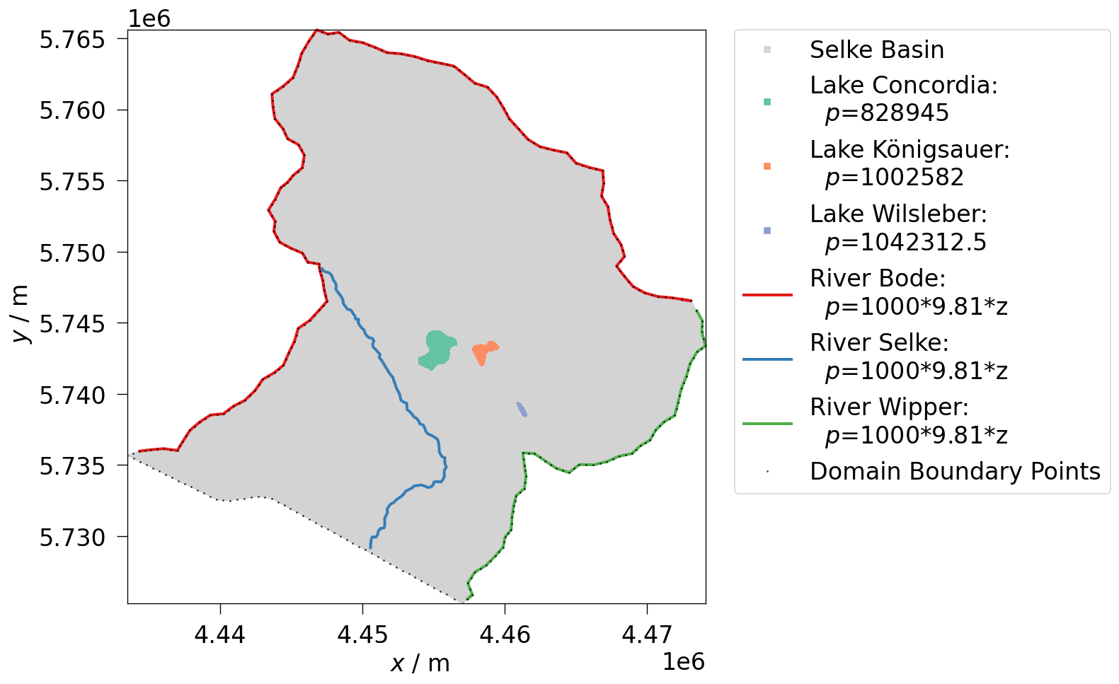
We can again visualise the boundary conditions and check that everything has been set up correctly.
model = ot.Model(project=project, meshes=meshes)…
(click to toggle)
model = ot.Model(project=project, meshes=meshes)

# Optional: Configure execution settings, e.g.
# model.execution.interactive = True # Uncomment for stepwise control

# Visualise boundary conditions
fig_constraints = model.plot_constraints(fontsize=20, show_edges=False, lw=0.6)
# Showing domain boundary points takes some additional effort
fig_constraints.axes[0].scatter(
    model.meshes["Selke_Basin_Domain_homo"].extract_feature_edges().points[:, 0],
    model.meshes["Selke_Basin_Domain_homo"].extract_feature_edges().points[:, 1],
    zorder=2,
    s=0.25,
)
fig_constraints.axes[0].plot(
    [], [], "s", label="Domain Boundary Points", c="black", ms=0.25
)
handles, labels = fig_constraints.axes[0].get_legend_handles_labels()
labels = [text.get_text() for text in fig_constraints.axes[0].legend_.get_texts()]
labels.append("Domain Boundary Points")
fig_constraints.axes[0].legend(
    handles=handles,
    labels=labels,
    loc="upper left",
    bbox_to_anchor=(1.05, 1),
    fontsize=20,
    borderaxespad=0.0,
    numpoints=1,
)<matplotlib.legend.Legend at 0x7f9bdc598440>
3. Run simulation
Running the simulation is now just as easy.
sim = model.run()…
(click to toggle)
sim = model.run()
# Optional: Check simulation status (i.e. if the simulation was successful)
print(f"Simulation status: {sim.status_str}")
assert sim.status == ot.Simulation.Status.doneSimulation status: Status: completed successfully (results available)
4. Analyse result
The results of the modelling process can be accessed through sim.meshseries.
Ogstools also already has some functions to further analyse the model output, allowing us to both see the process variables on the whole domain at any given time and to show the changes at a single point over the whole simulation interval.
Before we start plotting our results, we rescale the resulting mesh-series from SI-units into more readable ones.
sim.meshseries.scale(spatial="km", time="d")MeshSeries(filepath='/tmp/ogstools_gitlab-runner/MeshSeries/20260917_154802_956166/default.pvd', spatial_unit='km', time_unit='d')
StorageBase(id='20260917_154802_956166', is_saved=False, _active_target=None, next_target=PosixPath('/tmp/ogstools_gitlab-runner/MeshSeries/20260917_154802_956166/default.pvd'))
data_type='.pvd'
num_timesteps=11
dim=2
cached_meshes=1
4.1 Visualise final state
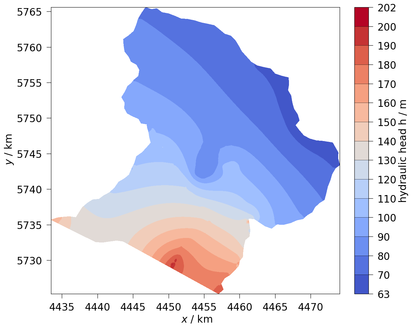
The example below shows hydraulic head at the last simulation interval.
Since we carried out the simulation using pressure as process variable we first have to create a new field containing the hydraulic head at each point.
After we have done this, we simply extract the mesh at our chosen time and plot it with the desired variable.
sim.meshseries.point_data["hydraulic head h / m"] = sim.meshseries.point_data[…
(click to toggle)
sim.meshseries.point_data["hydraulic head h / m"] = sim.meshseries.point_data[
    "pressure"
] / (1000 * 9.81)
fig = ot.plot.contourf(sim.meshseries[-1], "hydraulic head h / m", fontsize=20)
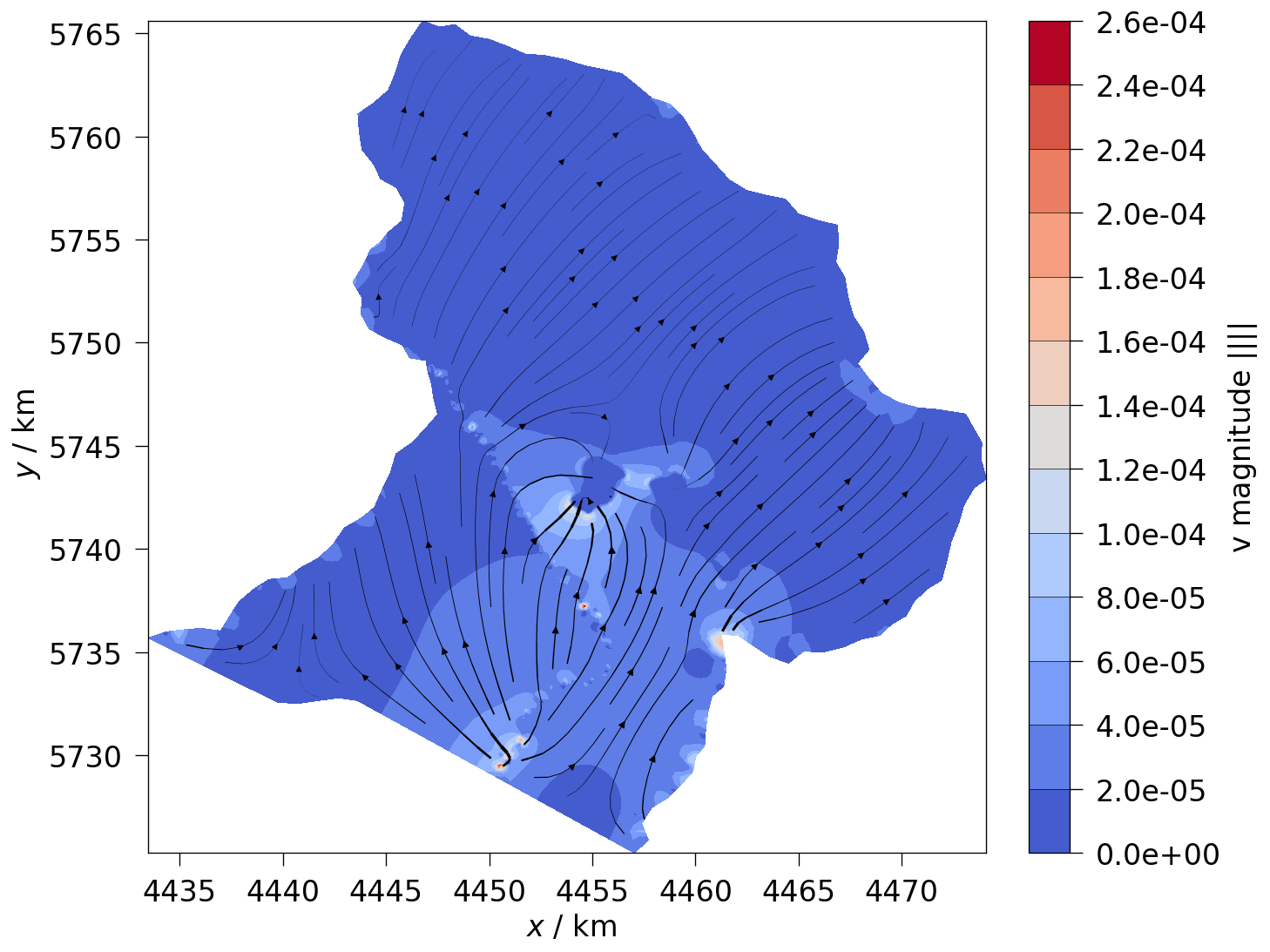
We can also see Darcy velocity
fig = ot.plot.contourf(sim.meshseries[-1], "v", fontsize=20)
4.2 Visualise process at single point
To do this, we first define the coordinates of our chosen observation point.
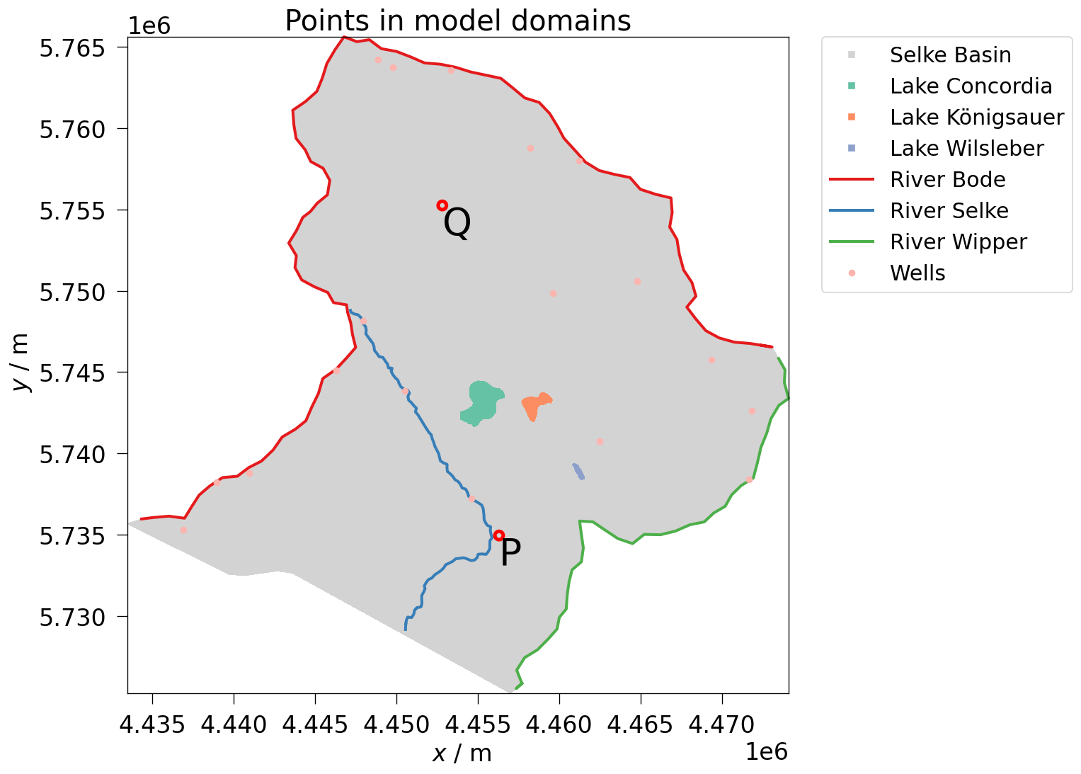
To check that we have chosen the correct coordinates we can plot the point into the meshes.
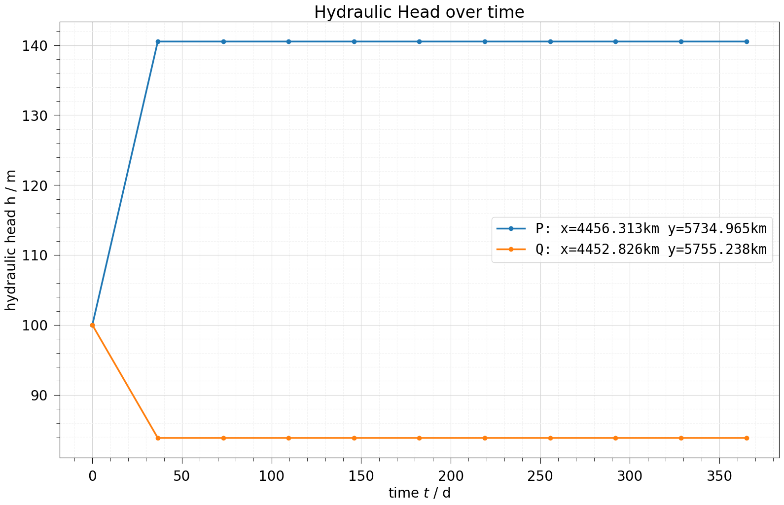
After that we extract the process variables for all times at the given point from the resulting mehseries using probe().
Finally we plot the extracted data as a line graph.
The example below shows the hydraulic head at x=4456.313 km, y=5734.965 km and x=4452.826 km, y=5755.238 km.
# Define points…
(click to toggle)
# Define points
point_P = (4456.313, 5734.965, 0.151)
point_Q = (4452.826, 5755.238, 0.153)
# Plot point
figpoint = meshes.plot(fontsize=20, show_edges=False, lw=0.6)
figpoint.axes[0].scatter(
    [point_P[0] * 1000, point_Q[0] * 1000],
    [point_P[1] * 1000, point_Q[1] * 1000],
    s=50,
    fc="none",
    ec="r",
    lw=3,
    zorder=2,
)
figpoint.axes[0].annotate("P", (4456313, 5734965), va="top", fontsize=32)
figpoint.axes[0].annotate("Q", (4452826, 5755238), va="top", fontsize=32)
figpoint.axes[0].set_title("Points in model domains", fontsize=24, loc="center")
# Extract data
probes = sim.meshseries.probe(np.array([point_P, point_Q]))
# Plot data
labels = [
    f"P: x={point_P[0]: >5}km y={point_P[1]}km",
    f"Q: x={point_Q[0]: >5}km y={point_Q[1]}km",
]
figline = probes.plot_line(
    "hydraulic head h / m", labels=labels, monospace=True, fontsize=20, marker="o"
)
figline.axes[0].set_title("Hydraulic Head over time", fontsize=24, loc="center")Text(0.5, 1.0, 'Hydraulic Head over time')
5. Run with different variables
Ogstools also contains built-in functions to manipulate existing projects. To do this we can use the replace_medium_property_value function to change the permeability of the medium and add_parameter and add_st to add a source term to the project.
To find more details on how writing and editing with ogstools works, see the following workflow
.
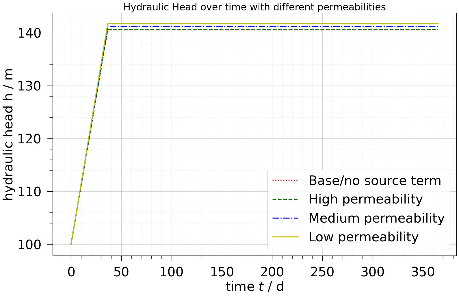
We will compare 4 scenarios: The above case without a source term and permeability $5.8\cdot 10^{-10}$, a low permeability case with added source term and permeability unchanged, a medium case with the source term and permeability $1\cdot 10^{-9}$ and a high permeability case with source term and permeability $1\cdot 10^{-8}$.
For each case we set up and run a separate model so that we can compare the changes in hydraulic head both at a chosen time over the whole domain and at our chosen point over the entire time.\
# Adding source term…
(click to toggle)
# Adding source term
project_source_term = project.copy()
project_source_term.parameters.add_parameter(
    name="q_recharge", type="Constant", value=3.18e-9
)
project_source_term.process_variables.add_st(
    process_variable_name="pressure",
    type="Volumetric",
    mesh="Selke_Basin_Domain_homo",
    parameter="q_recharge",
)
# Simulation high permeability…
(click to toggle)
# Simulation high permeability
project_hpm = project_source_term.copy()
project_hpm.replace_medium_property_value(0, "permeability", 1e-8)
model_hpm = ot.Model(project=project_hpm, meshes=meshes)
sim_hpm = model_hpm.run()
assert sim_hpm.status == ot.Simulation.Status.done
sim_hpm.meshseries.scale(spatial="km", time="d")
sim_hpm.meshseries.point_data["hydraulic head h / m"] = sim_hpm.meshseries.point_data[
    "pressure"
] / (1000 * 9.81)
# Simulation medium permeability…
(click to toggle)
# Simulation medium permeability
project_mpm = project_source_term.copy()
project_mpm.replace_medium_property_value(0, "permeability", 1e-9)
model_mpm = ot.Model(project=project_mpm, meshes=meshes)
sim_mpm = model_mpm.run()
assert sim_mpm.status == ot.Simulation.Status.done
sim_mpm.meshseries.scale(spatial="km", time="d")
sim_mpm.meshseries.point_data["hydraulic head h / m"] = sim_mpm.meshseries.point_data[
    "pressure"
] / (1000 * 9.81)
# Simulation low permeability…
(click to toggle)
# Simulation low permeability
project_lpm = project_source_term.copy()
model_lpm = ot.Model(project=project_lpm, meshes=meshes)
sim_lpm = model_lpm.run()
assert sim_lpm.status == ot.Simulation.Status.done
sim_lpm.meshseries.scale(spatial="km", time="d")
sim_lpm.meshseries.point_data["hydraulic head h / m"] = sim_lpm.meshseries.point_data[
    "pressure"
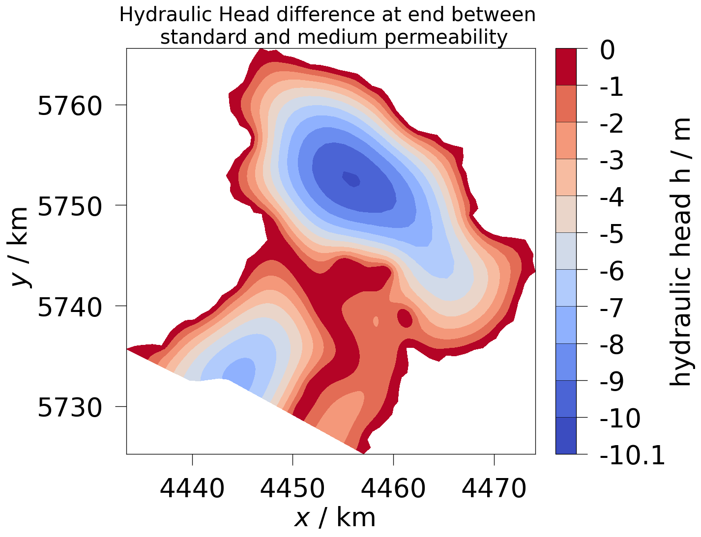
] / (1000 * 9.81)Having run our additional simulations, we can compute the differences in process variables between two meshseries and plot the results.
Here we show the difference between the base case (no source term, permeability $5.8\cdot 10^{-10}$) and the medium permeability case (added source term, permeability $1\cdot 10^{-9}$)
series_diff_mpm = ot.MeshSeries.difference(ms_a=sim.meshseries, ms_b=sim_mpm.meshseries)…
(click to toggle)
series_diff_mpm = ot.MeshSeries.difference(ms_a=sim.meshseries, ms_b=sim_mpm.meshseries)
fig_difference_mpm = ot.plot.contourf(series_diff_mpm[-1], "hydraulic head h / m")
fig_difference_mpm.axes[0].set_title(
    "Hydraulic Head difference at end between \n standard and medium permeability",
    fontsize=24,
    loc="center",
)Text(0.5, 1.0, 'Hydraulic Head difference at end between \n standard and medium permeability')
We can also show the changes in hydraulic head over the entire time at our previously chosen point P.
# Extract data from the new models…
(click to toggle)
# Extract data from the new models
probe_base = sim.meshseries.probe(point_P)
probe_hpm = sim_hpm.meshseries.probe(point_P)
probe_mpm = sim_mpm.meshseries.probe(point_P)
probe_lpm = sim_lpm.meshseries.probe(point_P)
# Plot all lines in one graph.
fig = probe_base.plot_line(
    "hydraulic head h / m",
    labels="Base/no source term",
    monospace=True,
    color="r",
    linestyle=":",
)
ax: plt.Axes = fig.axes[0]
ot.plot.line(
    probe_hpm,
    "hydraulic head h / m",
    ax=ax,
    label="High permeability",
    clip_on=False,
    color="g",
    linestyle="--",
)
ot.plot.line(
    probe_mpm,
    "hydraulic head h / m",
    ax=ax,
    label="Medium permeability",
    clip_on=False,
    color="b",
    linestyle="-.",
)
ot.plot.line(
    probe_lpm,
    "hydraulic head h / m",
    ax=ax,
    label="Low permeability",
    clip_on=False,
    color="y",
    linestyle="-",
)
fig.axes[0].set_title(
    "Hydraulic Head over time with different permeabilities", fontsize=24, loc="center"
)Text(0.5, 1.0, 'Hydraulic Head over time with different permeabilities')
# Check that simulations have produced expected outputs…
(click to toggle)
# Check that simulations have produced expected outputs
sim_end_expected = pv.read("expected_dirichlet.vtu")
np.testing.assert_allclose(
    sim.meshseries[-1]["pressure"], sim_end_expected["pressure"], atol=1e-10
)
hpm_end_expected = pv.read("expected_dirichlet_hpm.vtu")
np.testing.assert_allclose(
    sim_hpm.meshseries[-1]["pressure"], hpm_end_expected["pressure"], atol=1e-10
)
mpm_end_expected = pv.read("expected_dirichlet_mpm.vtu")
np.testing.assert_allclose(
    sim_mpm.meshseries[-1]["pressure"], mpm_end_expected["pressure"], atol=1e-10
)
lpm_end_expected = pv.read("expected_dirichlet_lpm.vtu")
np.testing.assert_allclose(
    sim_lpm.meshseries[-1]["pressure"], lpm_end_expected["pressure"], atol=1e-10
)OGS links
- Project file: Selke_Basin.prj
- Mesh files:
References
- Nixdorf, E., Sips, M., & Morstein, P. (2025). Development of a digital workflow for layer reduction strategies and visual-analytical outcome analysis to enhance geo-hydraulic modelling efficiency. Digital Water, 3(1), 1-24. doi:10.1080/28375807.2025.2460825