A 3-BHE Array Coupled With Pipe Network
Problem Description
For large-scale Ground Source Heat Pump (GSHP) systems, it is often coupled with an array of multiple Borehole Heat Exchangers in order to extract more heat from the subsurface. When operated over a long period of time, there can be thermal interference occurring among the BHEs. This can lead to thermal imbalance occurring in the subsurface. Since all BHEs are connected with each other through a pipeline network, the heat extraction rate on each individual BHE depends strongly on the inflow and outflow temperatures. As these temperature values were controlled by the pipeline network, it has an intrinsic feature of balancing thermal extraction rates among different BHEs. In order to quantitatively consider the thermal imbalance in the subsurface and the effect of the pipeline network, the calculation of hydraulic and heat transport in the pipe network must be included in the numerical simulation. This benchmark tests the pipe network feature with a 3D numerical model to show the phenomena of heat extraction rate shifting over a heating season. Since only 3 BHEs were included in this test, the percentage of shifted thermal load is limited. However, when dozens of BHEs are involved, the amount of shifted thermal load can be significant.
Model Setup
OGS
The BHE used in this Model contains a single U-shape pipe (1U type). The details about its finite element realisation could be found by Diersch et al. (2011). For the subsurface domain, a 50 $\times$ 50 $\times$ 72 $m$ mesh was constructed with prism and line elements. 3 BHEs are situated from -2 $m$ to a depth of -52 $m$ in the subsurface, with an adjacent distance of 6 $m$ from each other. The BHE #1 and BHE #3 are located at the left and right side, while the BHE #2 is installed in the centre. The initial soil temperature of the domain is set with 12 $^\circ$C. The top surface is assumed as Dirichlet boundary condition with a fixed temperature of 12 $^\circ$C over the entire simulation. To be noticed is that in this benchmark project file, the initial soil temperature and all boundary conditions are set to be 42 $^\circ$C, which is 30 $^\circ$C higher than they are described in the documentation. The reason for this is to prevent the circulation fluid (water) from freezing when calculating the TESPy pipe network model. The freezing of circulation fluid will actually lead to unexpected results in the TESPy solver (causing an enthalpy calculation error by the CoolProp library). Therefore all simulated temperature values are subtracted by 30 $^\circ$C before they are plotted and illustrated in the figures here. The detailed input parameters can be found in the 3bhes_1U.prj file, they are also listed in the following table.
| Parameter | Symbol | Value | Unit |
|---|---|---|---|
| Soil thermal conductivity | $\lambda_{s}$ | $2.4$ | $\mathrm{W m^{-1} K^{-1}}$ |
| Soil density | $\rho_{s}$ | $1120$ | $\mathrm{Kg m^{-3}}$ |
| Soil specific heat capacity | $(\rho c)_{s}$ | $2.0\times10^{6}$ | $\mathrm{J m^{-3}K^{-1}}$ |
| Length of the BHE | $L$ | $50$ | $\mathrm{m}$ |
| Diameter of the BHE | $D$ | $0.13$ | $\mathrm{m}$ |
| Diameter of the U-pipe in BHE | $d$ | $0.013665$ | $\mathrm{m}$ |
| Wall thickness of the pipe | $b_0$ | $0.003035$ | $\mathrm{m}$ |
| Wall thermal conductivity | $\lambda_{0}$ | $0.39$ | $\mathrm{W m^{-1} K^{-1}}$ |
| Grout thermal conductivity | $\lambda_{g}$ | $0.806$ | $\mathrm{W m^{-1} K^{-1}}$ |
| Grout heat capacity | $(\rho c)_{g}$ | $3.8\times10^{6}$ | $\mathrm{J m^{-3}K^{-1}}$ |
| Circulating fluid density | $\rho_{f}$ | $992.92$ | $\mathrm{Kg m^{-3}}$ |
| Circulating fluid thermal conductivity | $\lambda_{f}$ | $0.62863$ | $\mathrm{W m^{-1} K^{-1}}$ |
| Circulating fluid heat capacity | $(\rho c)_{f}$ | $4.16\times10^{6}$ | $\mathrm{J m^{-3}K^{-1}}$ |
| Length of the BHE U-pipe in network | $l$ | $100$ | $\mathrm{m}$ |
| Roughness coefficient of the pipe | $k_s$ | $0.00001$ | $\mathrm{m}$ |
TESPy
Here, the TESPy software developed by Francesco Witte is employed to simulate the coupled thermal-hydraulic status of a pipe network, which is composed of pre-defined components including pipes, heat exchangers, and different types of turbo machinery. Interested readers may refer to the online documentation of TESPy for the detailed introduction of the software. The TESPy version 0.3.2 is used in this benchmark.
Two different pipe network setup were constructed for this benchmark.
A one-way pipe network (see Figure 1)
In this setup, the refrigerant mass flow rate is given in $kg/s$, as this is the default setting in the TESPy model (see ./pre/3bhes.py).
After being lifted by the pump, the refrigerant inflow will be divided into 3 branches by the splitter and then flow into each BHEs.
Because of this configuration, the inflow temperature on each BHE will be the same.
The refrigerant flowing out of the BHEs array will be firstly mixed at the merging point and then extracted for the heat extraction through the heat pump.
After that, the refrigerant will flow out from the network.
For the boundary condition, a constant thermal load of 3750 $W$ is imposed on the heat pump over the entire simulation period.
In this case, the fluid enthalpy value at the splitter point is set to be equal to the sink point enthalpy, that means all the consumed heat on the heat pump is supplied by the BHEs array.
During the calculation of the TESPy solver, the flow density and the related specific heat capacity in the pipe network are automatically adjusted by calling the CoolProp library.
To check their concrete value under specific temperature and pressure conditions, interested readers may refer to e.g. the ‘PropsSI’ function introduced in the webpage of CoolProp.
For the fast execution of this benchmark, the total simulation time is shorten to 600 seconds. If the reader wishes to reproduce the same results, a full simulation of 6 months needs to be performed.

One-way pipeline network model
A closed-loop pipe network (see Figure 2)
The setup for a closed-loop network model is illustrated in Figure 1b. Compared to the configuration in the one-way network, the refrigerant in the closed loop network is circulating through the entire system. In this case, the flow rate will be automatically adjusted by the water pump in each time step, as its pressure head is directly linked to the flow rate. Subsequently, the flow rate is determined by the pressure losses in the BHE array.

Closed-loop pipeline network model
Results
The evolution of the soil temperature at 1 m distance away from the 3 BHEs are shown in Figure 3. Compared with the BHE #1 and BHE #3, the soil temperature near the BHE located at the centre (BHE #2) shows a deeper draw-down. It indicates that a thermal imbalance is occurring in the center of the BHE array. This imbalance leads to a lower outflow temperature from the BHE #2, which is shown in Figure 4. Figure 5 depicts the evolution of the heat extraction rate of each BHE over the time. Compared to the decrease of the heat extraction rate on the centre BHE #2, the rates on the other two BHEs located at the out sides was gradually increasing. It indicates that the heat extraction rate is shifting from the centre BHE towards the outer BHEs over the heating season. In this figure, the difference between the total heat extraction rate of all BHEs and the preset 3750 $W$ imposed on the heat pump is due to the hydraulic loss within each pipe in the pipe network.
In comparison to the one-way setup, the closed-loop network shows a slightly different behaviour. The evolution of inflow refrigerant temperature and flow rate entering the BHE array is shown in Figure 6. With the decreasing of the working fluid temperature over the time, the system flow rate decreases gradually. Figure 7 depicts the thermal load shifting phenomenon with the closed-loop model. Except for the thermal shifting behavior among the BHEs, the averaged heat extraction rate of all BHEs (black line) increases slightly over the time. This is due to the fact that additional energy is required to compensate the hydraulic loss of the pipe.
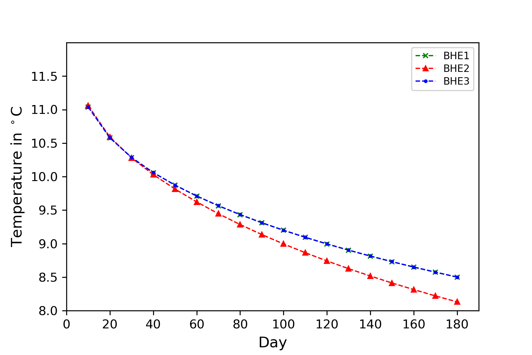
Evolution of the soil temperature located at the 1 m distance away from each BHE
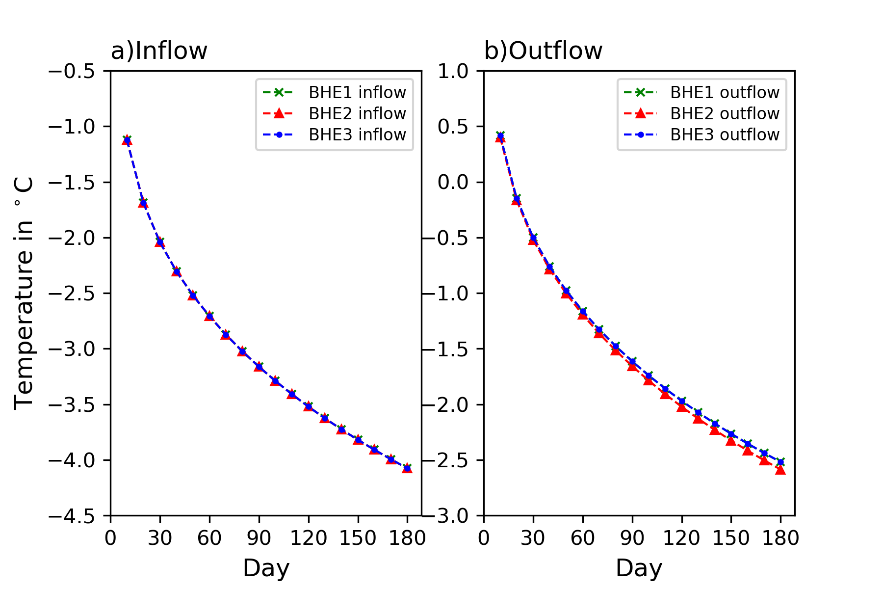
Evolution of the inflow and outflow refrigerant temperature of each BHE
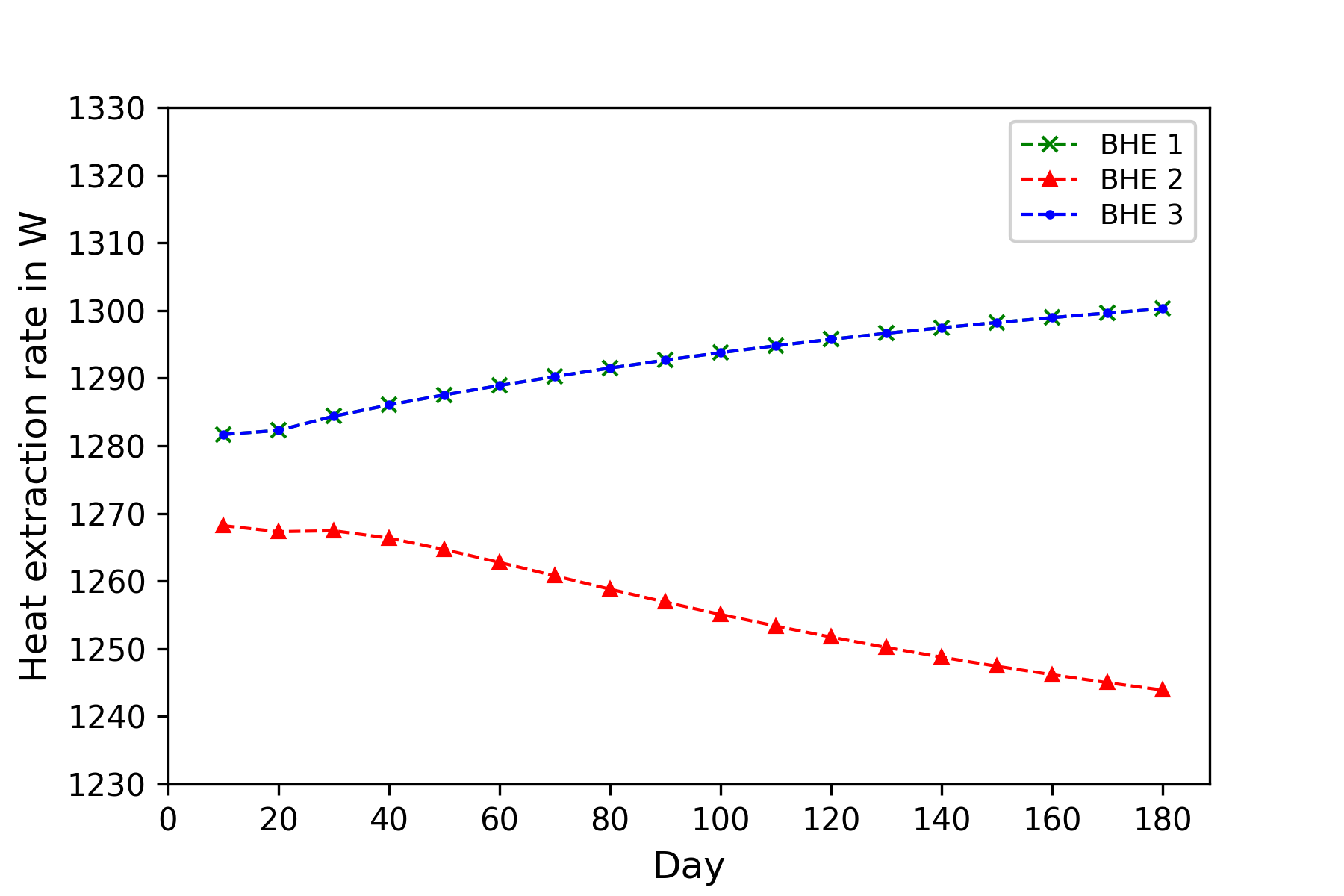
Evolution of the heat extraction rate of each BHE
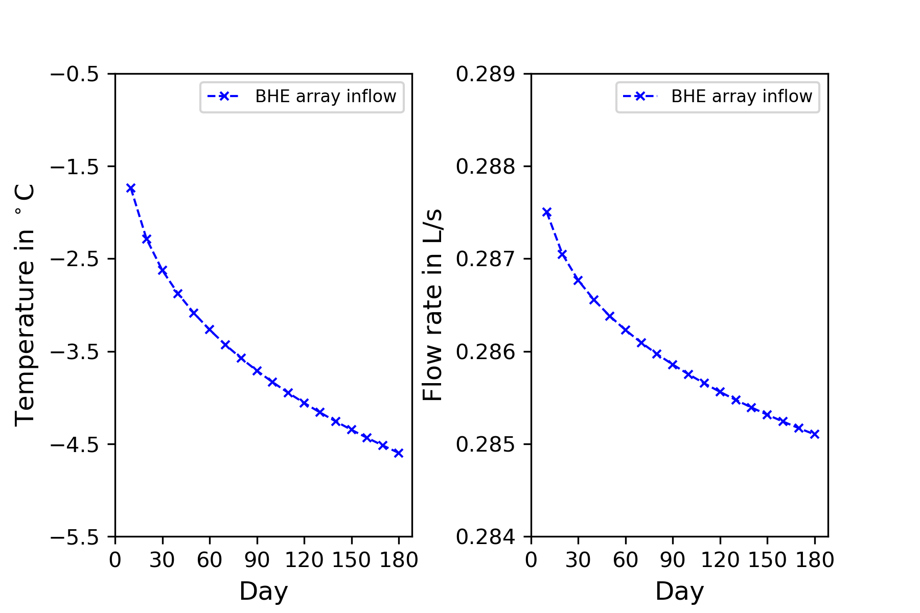
Evolution of the inflow refrigerant temperature and flow rate entering the BHE array
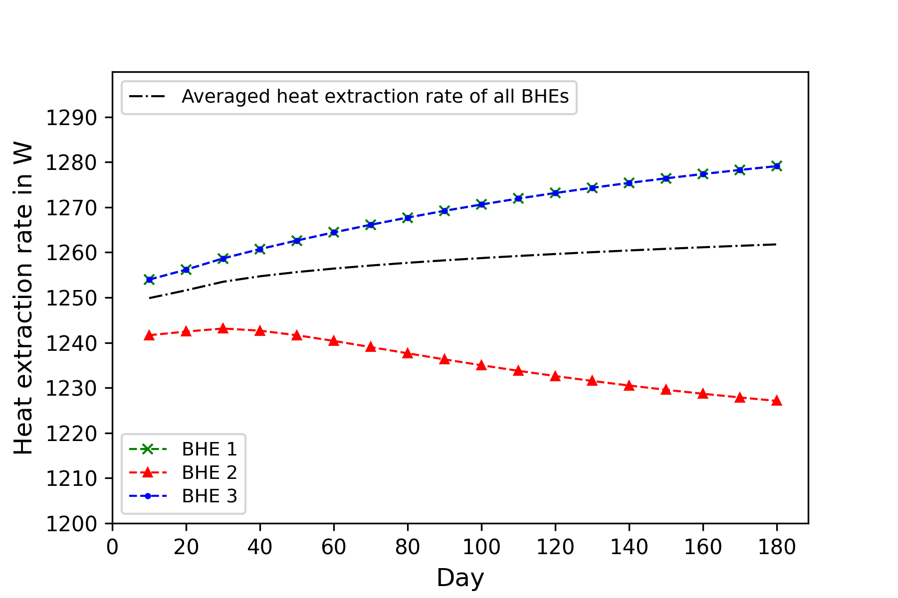
Evolution of the heat extraction rate of each BHE with close loop network model
References
[1] Diersch, H. J., Bauer, D., Heidemann, W., Rühaak, W., & Schätzl, P. (2011). Finite element modeling of borehole heat exchanger systems: Part 1. Fundamentals. Computers & Geosciences, 37(8), 1122-1135.
[2] Francesco Witte, Ilja Tuschy, TESPy: Thermal Engineering Systems in Python, 2019. URL: https://doi.org/10.21105/joss.02178. doi:10.21105/joss.02178.
[3] Webpage of the High-Level Interface in CoolProp. URL: http://www.coolprop.org/coolprop/HighLevelAPI.html.
This article was written by Shuang Chen, Haibing Shao. If you are missing something or you find an error please let us know.
Generated with Hugo 0.150.1
in CI job 743172
|
Last revision: February 5, 2026
Commit: [py,cmake] Allow Python 3.14. 4d949dd99c
| Edit this page on