3D 2U BHE
Model Setup
The numerical model was established based on dual continuum method developed by Diersch et al. (2011). In the 3D 2U type BHE benchmark, the depth of the whole domain is 18.5 m with a square cross section of 5 m per side. The BHE bottom is situated at -18 m and its total length is 18 m. Detailed parameters for the model configuration are listed in the following table.
| Parameter | Symbol | Value | Unit |
|---|---|---|---|
| Soil thermal conductivity | $\lambda_{s}$ | 2.78018 | $\mathrm{W m^{-1} K^{-1}}$ |
| Soil heat capacity | $(\rho c)_{soil}$ | $3.2\times10^{6}$ | $\mathrm{Jm^{-3}K^{-1}}$ |
| Length of the BHE | $L$ | 18 | $\mathrm{m}$ |
| Diameter of the BHE | $D$ | 0.13 | $\mathrm{m}$ |
| Diameter of the pipeline | $d$ | 3.78 | $\mathrm{cm}$ |
| Wall thickness of the pipeline | $b$ | 0.29 | $\mathrm{cm}$ |
| Distance between pipelines | $w$ | 5.3 | $\mathrm{cm}$ |
| Pipeline wall thermal conductivity | $\lambda_{p}$ | 0.42 | $\mathrm{W m^{-1} K^{-1}}$ |
| Grout thermal conductivity | $\lambda_{g}$ | 1 | $\mathrm{W m^{-1} K^{-1}}$ |
| Grout heat capacity | $(\rho c)_{grout}$ | $2.5\times10^{6}$ | $\mathrm{Jm^{-3}K^{-1}}$ |
OGS Input Files
For this benchmark, Two different scenarios were carried out by applying two different boundary conditions imposed on the BHE.
- Fixed inflow boundary condition
The detailed input parameters can be seen from the 3D_2U_BHE.prj file. The inflow temperature of the BHE, which was imposed as boundary condition of the BHE is shown in Figure 1. All the initial temperatures are set as 22 $^{\circ}$C. The flow rate within each U-pipe is set to $2.0\times10^{-4}$ $\mathrm{m^{3} s^{-1}}$ during the whole simulation time.
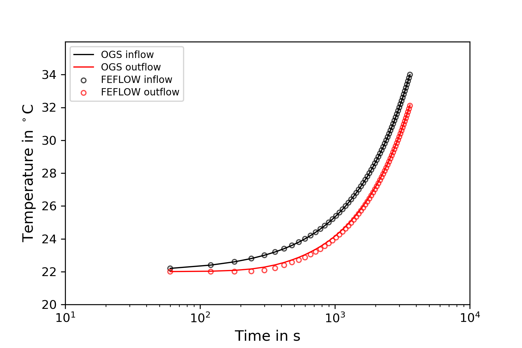
Figure 1: Inflow temperature curve and outflow temperature comparison
- Fixed power boundary condition
The detailed input parameters can be seen from the 3D_2U_BHE_powerBC.prj file. A -315.72 $W$ thermal load is imposed on the BHE to extract the heat from the subsurface during the entire simulation. All the other parameters adopted in the model is same as the ones used in the scenario with fixed inflow boundary condition.
FEFLOW Input Files
For the benchmark a FEFLOW model is presented. The mesh used in the OGS model is directly converted from the FEFLOW model mesh, to ensure that there is no influence to the comparison results from the mesh side. Both the FEFLOW and OGS model mesh can be found in the OGS GitLab (https://gitlab.opengeosys.org/ogs/ogs/-/merge_requests/3426).
FEFLOW Input Files
Results
The computed results from scenario by adopting the fixed inflow boundary condition are illustrated in Figure 1 and Figure 2. The OGS numerical outflow temperature over time was compared against results of the FEFLOW software as shown in the Figure 1. And the vertical distributed temperature of circulating water was presented in Figure 2 after operation for 3300 s. The comparison figures demonstrate that the OGS numerical results and FEFLOW results can match very well and the biggest absolute error of outflow temperature is 0.20 $^{\circ}$C after 360 s’ operation, while such error decreases to 0.037 $^{\circ}$C after 3600 s’ operation. The maximum relative error of vertical temperature is 0.019 % after operation for 3300 s.
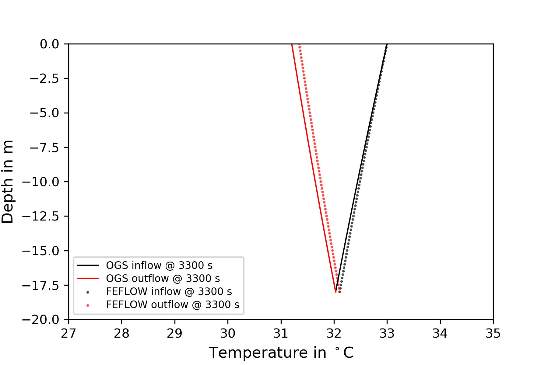
Figure 2: Comparison of vertical temperature distribution from scenario by adopting the fixed inflow boundary condition
Figure 3 shows the vertical distributed temperature of circulating fluid after operation for 3300 s by adopting different power boundary conditions in OGS and FEFLOW models.
Compared to the results computed from the OGS model with using a fixed power boundary condition (illustrated as the blue and green line), A 0.18 $^{\circ}$C difference is found for the averaged vertical temperature from the FEFLOW model (illustrated as the dotted line).
The reason to the results difference is due to the different power boundary condition type adopted in the two software.
In FEFLOW the power boundary condition is based on the outlet temperature calculated from the last time step (non-iterative).
Compared to it, the default power boundary condition adopted in the OGS Heat_Transport_BHE process is based on the outlet temperature calculated from the current time step (with-iterative).
Besides, by setting python bindings, the current OGS Heat_Transport_BHE process is capable to adopt the power boundary condition type used in the FEFLOW software.
In this way, the computed vertical distributed circulating fluid temperature is updated to the black and red solid line illustrated in the figure 3.
It shows that in this case, the difference between the OGS and FEFLOW models is becoming much closer to each other, which is about 0.037 $^{\circ}$C.
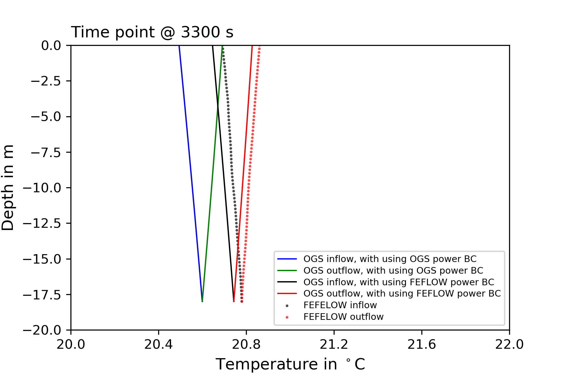
Figure 3: Comparison of vertical temperature distribution from scenarios by adopting the power boundary conditions
References
[1] Diersch, H. J., Bauer, D., Heidemann, W., Rühaak, W., & Schätzl, P. (2011). Finite element modeling of borehole heat exchanger systems: Part 1. Fundamentals. Computers & Geosciences, 37(8), 1122-1135.
[2] FEFLOW online documentation. URL: http://www.feflow.info/html/help72/feflow/14_References/GUI/Dialogs/bhe_editor.html.
This article was written by Chaofan Chen, Shuang Chen, Haibing Shao. If you are missing something or you find an error please let us know.
Generated with Hugo 0.150.1
in CI job 743172
|
Last revision: February 5, 2026
Commit: [py,cmake] Allow Python 3.14. 4d949dd99c
| Edit this page on