Solute transport including kinetic reaction
Overview
This scenario describes the transport of two solutes (Synthetica and Syntheticb) through a saturated media. Both solutes react to Productd according to $\text{Product d}=\text{Synthetic a}+0.5~\text{Synthetic b}$. The speed of the reaction is described with a first–order relationship $\frac{dc}{dt}=U(\frac{c_{\text{Synthetic a}}}{K_m+c_{\text{Synthetic b}}})$. The coupling of OGS-6 and IPhreeqc used for simulation requires to simulate the transport of $H^+$–ions, additionally. This is required to adjust the compulsory charge balance computation executed by Phreeqc. The solution by OGS-6–IPhreeqc will be compared to the solution by a coupling of OGS-5–IPhreeqc.
Problem Description
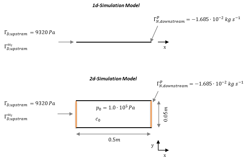
1d scenario: The 1d–model domain is 0.5 m long and discretised into 200 line elements. The domain is saturated at start–up ($p(t=0)=$ 1.0e-5 Pa). A constant pressure is defined at the left side boundary ($g_{D,\text{upstream}}^p$) and a Neumann BC for the water mass out-flux at the right side ($g_{N,\text{downstream}}^p$). Both solutes, Synthetic a and Synthetic b are present at simulation start–up at concentrations of $c_{\text{Synthetic a}}(t=0)=c_{\text{Synthetic b}}(t=0)= 0.5~\textrm{mol kg}^{-1}~\textrm{water}$, the influent concentration is $0.5~\textrm{mol kg}^{-1}~\textrm{water}$ as well. Product d is not present at start–up ($c_{\text{Productd}}(t=0)=0$); neither in the influent. The initial concentration of $\text{H}^+$–ions is $1.0e\textrm{-}7~\textrm{mol kg}^{-1}~\textrm{water}$; the concentration at the influent point is the same. Respective material properties, initial and boundary conditions are listed in the tables below.
2d scenario: The 2d–scenario only differs in the domain geometry and assignment of the boundary conditions. The horizontal domain is 0.5 m in x and 0.5 m in y direction, and, discretised into 10374 quadratic elemtents with an edge size of 0.0025 m.
| Parameter | Description | Value | Unit |
|---|---|---|---|
| $\phi$ | Porosity | 1.0 | |
| $\kappa$ | Permeability | 1.157e-12 | $\textrm{m}^2$ |
| $S$ | Storage | 0.0 | |
| $a_L$ | long. Dispersion length | 0.0 | m |
| $a_T$ | transv. Dispersion length | 0.0 | m |
| $\rho_w$ | Fluid density | 1.0e+3 | $\textrm{kg m}^{-3}$ |
| $\mu_w$ | Fluid viscosity | 1.0e-3 | Pa s |
| $D_{\text{H}^+}$ | Diffusion coef. for $\text{H}^+$ | 1.0e-7 | m$^2$ s |
| $D_{solutes}$ | Diffusion coef. for Synthetica, Syntheticb and Productd | 1.0e-12 | m$^2$ s |
| $U$ | Reaction speed constant | 1.0e-3 | h$^{-1}$ |
| $K_m$ | Half–saturation constant | 10 | mol kg$^{-1}$ water |
Table: Media, material and component properties
| Parameter | Description | Value | Unit |
|---|---|---|---|
| $p(t=0)$ | Initial pressure | 1.0e+5 | Pa |
| $g_{N,downstream}^p$ | Water outflow mass flux | -1.685e-02 | mol kg$^{-1}$ water |
| $g_{D,upstream}^p$ | Pressure at inlet | 1.0e+5 | Pa |
| $c_{Synthetica}(t=0)$ | Initial concentration of Synthetica | 0.5 | mol kg$^{-1}$ water |
| $c_{Syntheticb}(t=0)$ | Initial concentration of Syntheticb | 0.5 | mol kg$^{-1}$ water |
| $c_{Productd}(t=0)$ | Initial concentration of Productd | 0 | mol kg${^-1}$ water |
| $c_{\text{H}^+}(t=0)$ | Initial concentration of $\text{H}^+$ | 1.0e-7 | mol kg$^{-1}$ water |
| $g_{D,upstream}^{Synthetica_c}$ | Concentration of Synthetica | 0.5 | mol kg$^{-1}$ water |
| $g_{D,upstream}^{Syntheticb_c}$ | Concentration of Syntheticb | 0.5 | mol kg$^{-1}$ water |
| $g_{D,upstream}^{Productd}$ | Concentration of Productd | 0.0 | mol kg$^{-1}$ water |
| $g_{D,upstream}^{\text{H}^+}$ | Concentration of $\text{H}^+$ | 1.0e-7 | mol kg$^{-1}$ water |
Table: Initial and boundary conditions
Results
The kinetic reaction results in the expected decline of the concentration of Synthetic a and Synthetic b, which is super-positioned by the influx of these two educts through the left side.
By contrast, the concentration of Product d increases in the domain.
Over time, opposed concentration fronts for educts and Product d evolve.
Both, OGS-6 and OGS-5 simulations yield the same results in the 1d as well as 2d scenario.
For instance, the difference between the OGS-6 and the OGS-5 computation for the concentration of Product d expressed as root mean squared error is 1.76e-7 mol kg$^{-1}$ water (over all time steps and mesh nodes, 1d scenario); the corresponding median absolute error is 1.0e-7 mol kg$^{-1}$ water.
This verifies the implementation of OGS-6–IPhreeqc.
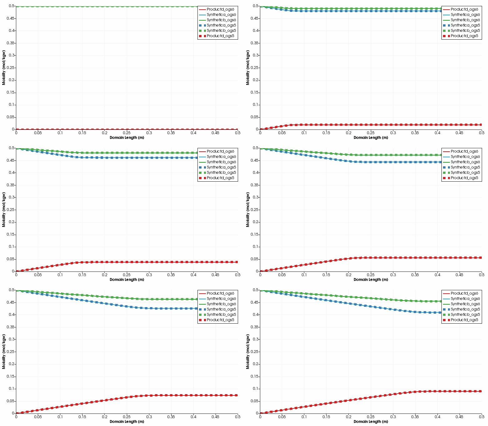
Simulated component concentrations over domain length for different time steps (1d scenario) .
 Community Discussion
The following comments are pulled in from our Discourse forum and contain community-generated content.
This article was written by Johannes Boog. If you are missing something or you find an error please reach out
to us on our forum.
Generated with Hugo 0.164.0
in CI job 825193
|
Last revision: April 20, 2026
Commit: refactor(MeshLib): remove PropertyVector::push_back 870422dde
| Edit this page on