BGRa creep model

• ThermoMechanics/CreepBGRa/SimpleAxisymmetricCreep/SimpleAxisymmetricCreepWithAnalyticSolution.prj

The BGRa stationary creep model defines the uniaxial creep strain increment as

where $\sigma_1$ is the stress, $A$, $m$ and $Q$ are parameters determined by experiments, $Q$ is called activation energy, $R_u=8.314472 \mbox{J/(Kmol)}$ is the universal gas constant, and ${ \sigma}_f$ is a stress scaling factor.

Creep potential and creep strain

Assume there is a creep potential $g^c$ and the creep induced strain rate is given by the flow rule

where ${ \mathbf\sigma}$ is the stress tensor. To establish equivalence between the three-dimensional and the uniaxial formulation given above, we use the effective stress defined by ${ \bar\sigma}={\sqrt{{\frac{3}{2}}}}{\left\Vert{\mathbf s}\right\Vert}$ with ${\mathbf s}= { \mathbf \sigma}-\frac{1}{3}{ \mathrm{tr}(\mathbf\sigma}){\mathbf I}$, the deviatoric stress. The creep strain rate is then expressed as

The above creep strain rate expression must be valid for problems independent from the Euclidean dimension. Applying the creep rate equation to a uniaxial stress state ${\mathbf \sigma} = \mathrm{diag}[\sigma_1, 0, 0]$, which gives ${\mathbf s} = \mathrm{diag}[\frac{2}{3}\sigma_1, -\frac{1}{3}\sigma_1, -\frac{1}{3}\sigma_1]$, we have

which says

Therefore, the creep strain rate for multi-dimensional problems can be derived as

Stress integration

The above creep strain rate expression can be simplified as

with

The strain rate under creeping condition can be expressed as

Due to Hook’s law, the stress rate is given by

where $\mathbf{C} = \lambda \mathcal{I} + 2G \mathbf I \otimes \mathbf I$ with $\mathcal{I}$ the fourth order identity, $\mathbf I$ the second order identity, $\lambda$ the Lamé constant, $G$ the shear modulus, and $\otimes$ the tensor product notation.

is a fourth order tensor. Substituting equation and the expression of $C$ into the stress rate expression, equation, we have

The stress of the present time step, $n+1$, is then can be expressed as

with $\alpha_T$ the linear thermal expansion.

To solve the stress, the Newton-Raphson is applied. Let

be the residual. The Jacobian of is derived as

Consistent tangent

Once the converged stress integration is obtained, the tangential of stress with respect to strain can be obtained straightforwardly by applying the partial derivative to equation with respect to strain increment as

We see that

If the model is used for the thermo-mechanical problems and the problems are solved by the monolithic scheme, the displacement-temperature block of the global Jacobian can be derived as $$\begin{aligned}

-2G\dfrac{Q}{R} {{\int}_{\Omega} \dfrac{b}{T^2} {\left\Vert{\mathbf s}^{n+1}\right\Vert}^{m-1} \mathbf{B}^T {\mathbf s}^{n+1} \mathrm{d} \Omega} \end{aligned}

Note: The above rate form of stress integration is implemented in OGS. Alternatively, one can use an absolute stress integration form, which can be found in the attached PDF.

Example

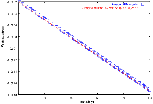
We verify the scheme by a one dimensional extension with constant pressure of ${ \sigma}_0=5 ~\mbox{MPa}$. The values of the parameters are given as $A=0.18 \mbox{d}^{-1}$, $m=5$, $Q=54 ~\mbox{kJ/mol}$, $E=25000 ~\mbox{MPa}$, and the temperature is constant everywhere of 100 $^{\circ}\mbox{C}$. The analytical solution of the strain is given straightforward as

The problem is solved as an axisymmetric one. Therefore

Because of

we have

and

with $\epsilon^e=\epsilon-\epsilon^c$, where superscript $e$ means elasticity and $c$ means creep. With the creep strain formulas that are presented in the above context, the analytical solutions of the other main strains are

The comparison of the result of $\epsilon_z$ obtained by the present multidimensional scheme with the analytical solution is shown in the following figure:

Python code

A short python snippet, to compute the values.

A = self.GetInputDataObject(0, 0)
numPoints = A.GetNumberOfPoints()
outSxx = vtk.vtkDoubleArray()
outSxx.SetName('analytic_strain_xx')
outSyy = vtk.vtkDoubleArray()
outSyy.SetName('analytic_strain_yy')
outSzz = vtk.vtkDoubleArray()
outSzz.SetName('analytic_strain_zz')
outSxy = vtk.vtkDoubleArray()
outSxy.SetName('analytic_strain_xy')
sigma0=5.0
A=0.18
m=5
Q=54000
E=25000
R=8.314472
sf=1.
t=100
e0=-sigma0/E
c=-A*exp(-Q/(R*373.15))*pow(sigma0,m)
strain_zz=e0+c*t
nv=0.27
G=0.5*E/(1+nv)
strain_rr=strain_zz + 0.5*sigma0/G+1.5*A*exp(-Q/(R*373.15))*pow(sigma0, m)*t
for i in range(0, numPoints):
    outSxx.InsertNextValue(strain_rr)
    outSyy.InsertNextValue(strain_zz)
    outSzz.InsertNextValue(strain_rr)
    outSxy.InsertNextValue(0)
output = self.GetOutput()
output.GetPointData().AddArray(outSxx)
output.GetPointData().AddArray(outSyy)
output.GetPointData().AddArray(outSzz)
output.GetPointData().AddArray(outSxy)