Creep in a rectangle domain with hole under pressure on its top surface
Following up the benchmark about the BGRa creep model described on the this page, this example represents the creep in the near field of drift in the deep rock salt after excavation. The domain and the geometry are shown in the following figure:

The domain has two material groups, which are highlighted by different colors. The material group that is in the top part of the domain represents a cap rock type, while the other material group is for rock salt. The material properties of the rocks are given in the following table:
| Cap rock | Rock salt | Unit | |
|---|---|---|---|
| Density | 2000 | 2170 | kg/m$^{3}$ |
| Young’s Modulus | 7.0 | 7.65 | GPa |
| Poisson ratio | 0.3 | 2.7 | - |
| Thermal conductivity | 5 | 5 | W/(mK) |
The parameters of the BGRa creep model are $A=0.18\, \mbox{d}^{-1}$, $m=5$, $Q=54 \mbox{ kJ/mol}$ for the rock salt. For the cap rock, $A$ is set to zero.
The width and the height of the domain are 300 m and 340 m, respectively. The height of the cap rock portion is 40 m. The drift to be excavated has a radius of 50 m.
Here we consider the creep of the rock after excavation. Therefore, we assume a steady state of stress and temperature of excavation at the beginning of the current simulation. For this assumption, the boundary conditions are given as:
-
top boundary: $\tau_x =$$\sigma_x$$_y=0$, $\tau_y=\sigma_y=-10$ MPa, $T=310$ K.
-
two lateral boundaries: normal displacement is fixed, and no heat flux.
-
bottom boundary: normal displacement is fixed, and $T=320$ K.
-
circle of drift surface: traction free (${ \mathbf\sigma}\cdot \mathbf n = 0$), and $T=300$ K as excavation conditions.
The boundary conditions of the mechanical process lead to a distinct stress field after excavation. Besides, heat capacity is neglected in order to pose a steady state temperature field after excavation. The initial stresses are zero and the initial temperature is linearly distributed from top to bottom with the boundary values of temperature.
The time step sizes of the simulation are: One step of 0.001 day, 10 steps of 0.1 day, and the remaining steps of 1 day.
The following three figures are plotted by using the results of the simulation of 1000 days creep. The three figures display the distribution of horizontal and vertical stresses at times of 108 days, 409 days and 1000 days, respectively.
In these three figures, the left sub-figure show the time variations of horizontal and vertical stresses at a position just close to the top of the drift, and the green vertical line in it marks the time of the displayed stress field.
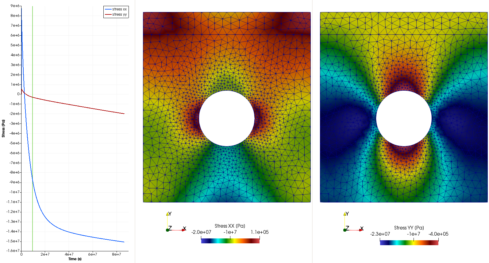
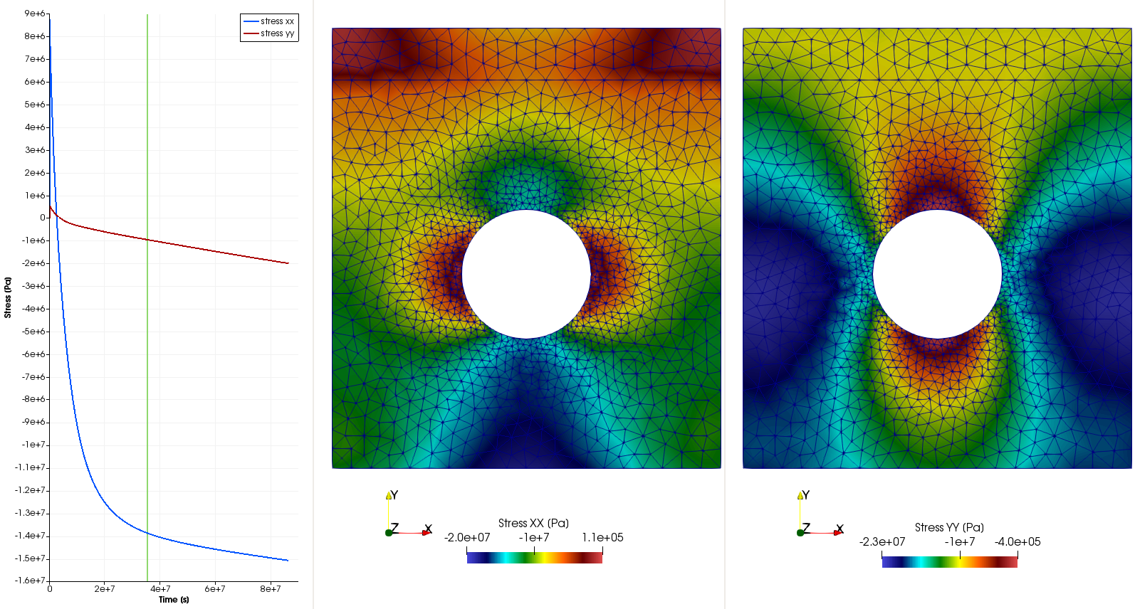
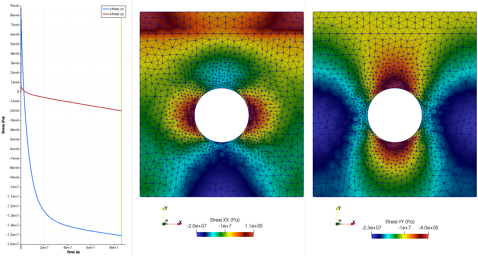
The above three figures show that the absolute value of the horizontal stress increase signification in the areas above and beneath the drift due to the creep, and the change of the vertical stress is slow compared to that of the horizontal stress.
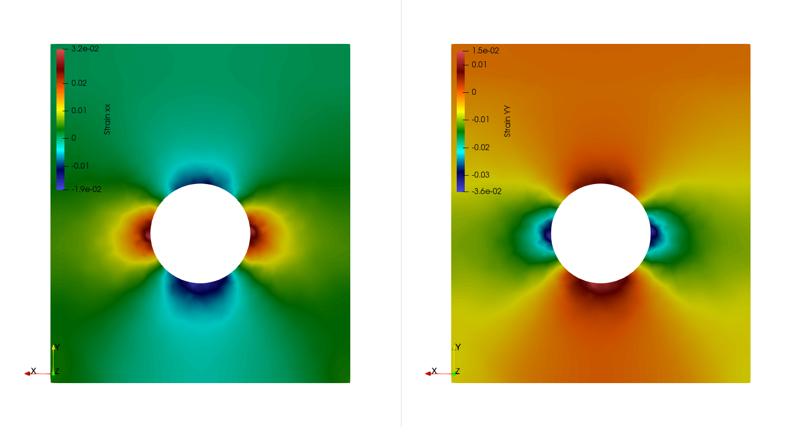
The following figure shows the strain distribution at the end of the simulation time at 1000 days.
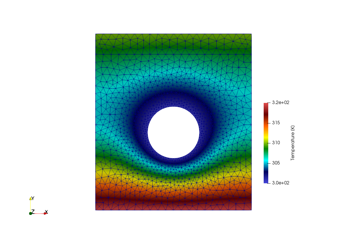
The steady-state temperature distribution is displayed in the following figure
Note
For the automatic benchmarking, the time duration of creep is reduced to 50 days in order to reduce the run time.
If one wants to test this benchmark for 1000 days’ creep, please change the end time in the tag of <t_end>
in the project file as
<t_end>86400.0e+3</t_end>This article was written by Wenqing Wang. If you are missing something or you find an error please let us know.
Generated with Hugo 0.150.1
in CI job 743172
|
Last revision: February 5, 2026
Commit: [py,cmake] Allow Python 3.14. 4d949dd99c
| Edit this page on