Checking the volumetric expansion due to water-to-ice phase change

• ThermoHydroMechanics/9percentWaterFreezingExpansion/UnitSquare.prj

Problem description

The aim of this benchmark is to verify that our THM model is capable of simulating the 9% volumetric expansion during the liquid-to-ice phase transition. This must be captured by the $\boldsymbol\sigma_\mathrm{I}$-stress component of the formulation

$$ \begin{align*} \boldsymbol\sigma\_\mathrm{SI} :=&\boldsymbol\sigma\_\mathrm{S}+ \boldsymbol\sigma\_\mathrm{I} \\\\\\ =&\mathbb{C}\_\mathrm{S}:\left(\boldsymbol\varepsilon-\alpha^\mathrm{S}\_T (T-T\_0){\bf I}\right) \\\\\\ +&\phi S\_\mathrm{I}(T) \mathbb{C}\_\mathrm{IR}: \left(\boldsymbol\varepsilon-\boldsymbol\varepsilon\_\mathrm{S0} - \alpha^\mathrm{I}\_T (T-T\_\mathrm{m}){\bf I} - \alpha\_{\phi\_\mathrm{I}} S\_\mathrm{I}(T){\bf I} \right), \end{align*} $$

where $\mathbb{C}\_\mathrm{S}$ and $\mathbb{C}\_\mathrm{IR}$ are the forth order elasticity tensors of solid matrix and ice phase, respectively, $\boldsymbol\varepsilon$ is the total strain, $\alpha^\mathrm{S}\_T$ and $\alpha^\mathrm{I}\_T$ are the linear thermal expansivities of solid and ice phases, respectively, $\phi$ is the porosity, $\alpha_{\phi_\mathrm{I}}=0.03$ is the linear expansion coefficient due to water-to-ice phase change and, finally, $S\_\mathrm{I}(T)$ is the regularized ice phase indicator function ($S\_\mathrm{I}\rightarrow 1$ is ice, and $\rightarrow 0$ is liquid water). Then the material properties in the benchmark are to be chosen such that $E_\mathrm{S}\ll E_\mathrm{IR}$. In this way, and also with the absence of mechanical loading, the deformation of a specimen — with $\alpha_{\phi_\mathrm{I}}$ being the strain increase in each space direction — will occur solely due to liquid freezing.

The material properties in the benchmark are to be chosen such that the Young’s modulus of solid is smaller than that of ice, i.e. $E_\mathrm{S}\ll E_\mathrm{IR}$. In this way, and also with the absence of mechanical loading, the deformation of a specimen with $\alpha_{\phi_\mathrm{I}}=0.03$ being the strain increase in each space direction will occur solely due to liquid freezing.

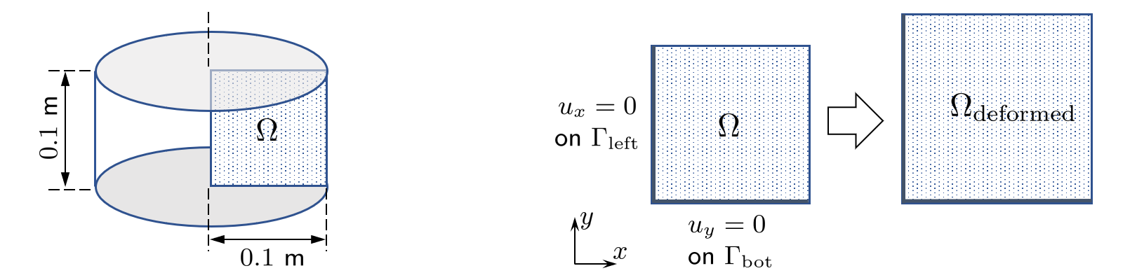
For the geometric setup we consider a fully saturated cylindrical column whose bottom edge is supported by a rigid foundation. Using the axis symmetry the problem is reduced from 3 to 2 dimensions with a simple (square) computational domain and related (Dirichlet) boundary conditions, see Figure 1, where an expected deformed configuration is also sketched. Again, we apply no mechanical loading to the specimen, whereas the thermal loading is presented by temperature evolution over time. The temperature $T$ is prescribed as a constant in $\Omega$ at each time step and decays linearly from $+4\\,^\circ \text{C}$ to $-4\\,^\circ \mathrm{C}$ during one hour term, as depicted in Figure 2, left.

Figure 1: Fully saturated column expansion due to water-to-ice phase transition: geometry (on the left) and the 2d computational setup along with the expected deformed configuration (on the right).

Material data used in the computations are presented in Table 1. No liquid phase parameters are present since we don’t solve for the hydraulic equation and the temperature field is prescribed. The two parameters that are varied are the time step increment $\Delta t$ (also denoted as $\mathrm{dt}$ in the corresponding captions) and the parameter $k>0$ in the Sigmoid function $S_\mathrm{I}$ which governs the “thickness” of a temperature-related phase transition zone. More specifically, we take $\Delta t\in\\{10\\,\mathrm{s}, 30\\,\mathrm{s}, 60\\,\mathrm{s}\\}$ and $k\in\\{2,5,20,50\\}$. $\Omega$ is discretized with only one element (which is possible/allowed here since the setup implies no freezing front propagation within the domain). Finally, the FE approximation of the components of strain tensor $\boldsymbol\varepsilon$ uses the $Q_1$-quadrilaterals.

Table: Material properties and parameters.

Simulation results and analysis

Figure 2, right, depicts evolution of strain tensor components $\varepsilon_{xx}$, $\varepsilon_{yy}$, $\varepsilon_{zz}$ computed for the fixed parametric pair $(\Delta t, k)=(60\\,\mathrm{s}, 20)$. All three strains behave identically and, more importantly, as expected, they transit from 0 to the reference magnitude of 0.03 during the freezing, in accordance to the term $\alpha_{\phi_\mathrm{I}}S_\mathrm{I}(T)$.

Figure 2: The prescribed temperature loading applied to the specimen (on the left) and the induced strains evolution due to phase change (on the right).

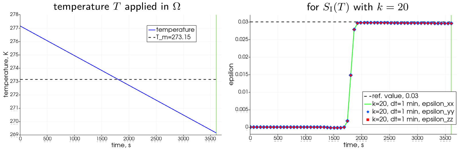
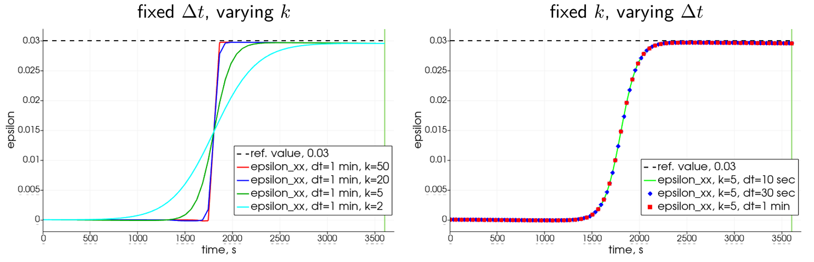
Figure 3 details the parametric studies for the computed $\varepsilon_{xx}$: on the left plot, for the fixed time increment, one observes that for any considered $k$ the corresponding strains transit up to the required value 0.03 and, as also expected, the increase of the parameter yields a steeper and more localized transition zone, almost mimicking the Heaviside-like behaviour at $k=50$. It is interesting to observe a slight downward deviation of $\varepsilon_{xx}$ from the horizontal reference value in the post-freezing time range (that is, when the prescribed temperature keeps on decreasing from $T_\mathrm{m}$ to $-4\\,^\circ\mathrm{C}$). This behaviour is physical and implies the ice contraction in such temperature range. The right plot of Figure 3 presents the evolution of $\varepsilon_{xx}$—specifically, the required transit during the phase change—for a fixed steepness-related parameter $k$ and varying time step size. All three computational results seem identical.

Figure 3: Parametric studies for the computed volumetric strain expansion in dependence on the time step size and parameter $k$ in $S_\mathrm{I}(T)$ that governs the thickness of the phase transition zone.