Fully saturated column deformation and freezing

• ThermoHydroMechanics/ColumnDeformationFreezing/TM.prj

Problem description

In this example, we consider a fully saturated poro-elastic column which is subject to a combination of thermal and mechanical loading. This loading is prescribed in a way that various stages and kinds of deformation process of the specimen such as purely mechanical deformation of the solid matrix, deformation of the solid-ice mixture, as well as deformation induced by the liquid-to-ice phase transition are present/envisioned. We thus verify the M+freezing model given by the IBVP problem for the momentum of balance equation.

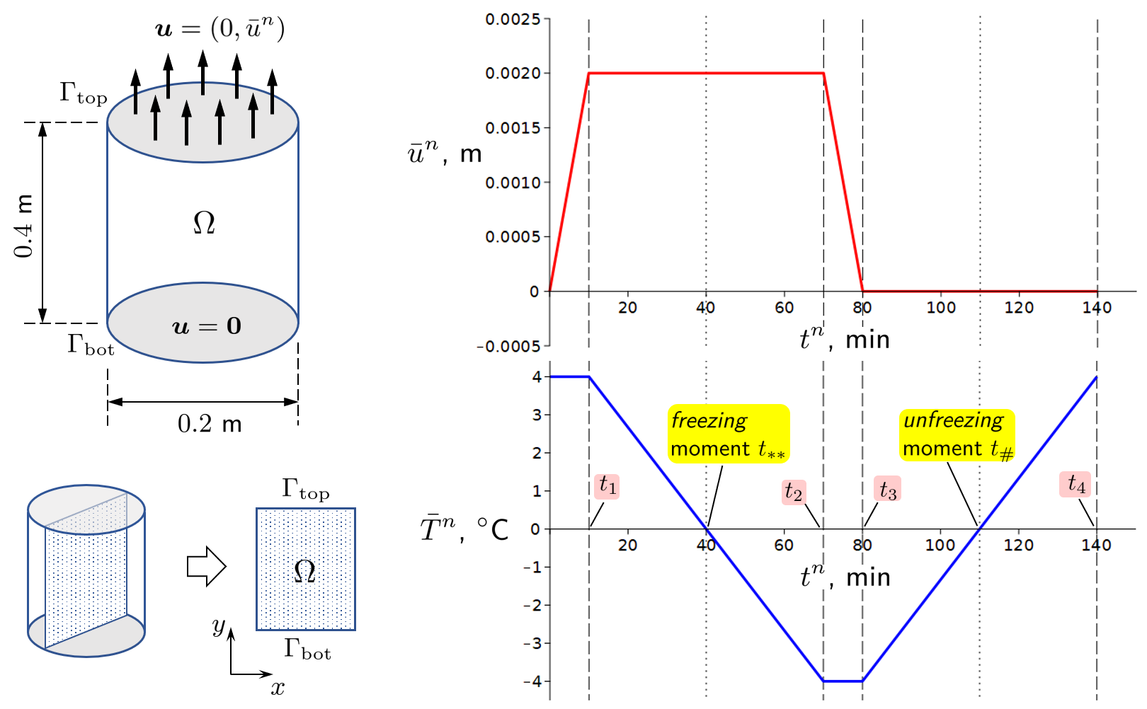
The left plot of Figure 1 depicts geometric and mechanical loading setup: the cylindrical column $\Omega$ is fixed at the bottom edge $\Gamma_\mathrm{bot}$ and the incremental vertical displacement loading $\bar{u}^n$, with $n\geq1$ being a time step, is applied at column’s top boundary $\Gamma_\mathrm{bot}$. Simultaneously, the incremental thermal loading $\bar{T}^n$ is applied within the column. This implies, that all temperature dependent coefficients in the moment balance equation are varied by setting $T=\bar{T}^n$ therein. Figure’s right plot details both $\bar{u}^n$ and $\bar{T}^n$ including the time intervals of interest. The unknown we solve for is the specimen displacement field $\boldsymbol u$. Notice that using the symmetry of the 3-dimensional domain, we effectively consider and solve the 2-dimensional problem in a diametrical cross-section.

Figure 1: Fully saturated poro-elastic column geometry and mechanical loading (on the left); plots of the prescribed displacement and thermal loading applied to the specimen (on the right).

Simulation results and analysis

To assess and analyse our simulation results, we calculate and record at each time step the vertical component $F_y$ of reaction force on the top boundary $\Gamma_\mathrm{top}$, namely,

$$ \boldsymbol F^n=(F^n_x,F^n_y):=\int_{\Gamma_\mathrm{top}} \boldsymbol\sigma(\boldsymbol u^n)\cdot\boldsymbol n\\, \mathrm{d}s \quad\text{for $\boldsymbol\sigma \in \\\{ \boldsymbol\sigma_\mathrm{S}, \boldsymbol\sigma_\mathrm{I}, \boldsymbol\sigma_\mathrm{SI} \\\}$}, $$

where $\boldsymbol u^n:\Omega\rightarrow\mathbb{R}^2$ is the computed displacement solution vector, and $\boldsymbol n$ is an outward normal on $\Gamma_\mathrm{top}$. The stresses shown in the Figure 2. are: the solid matrix stress $\boldsymbol\sigma_\mathrm{S}$, the pore ice fraction stress $\boldsymbol\sigma_\mathrm{I} := \phi_\mathrm{I}(T)\boldsymbol\sigma_\mathrm{IR}$, and the solid-ice mixture stress $\boldsymbol\sigma_\mathrm{SI}:=\boldsymbol\sigma_\mathrm{S}+\boldsymbol\sigma_\mathrm{I}$.

Figure 2: Plots of the vertical reaction force $F_y^n$ for the solid matrix, pore-ice and the solid-ice mixture.

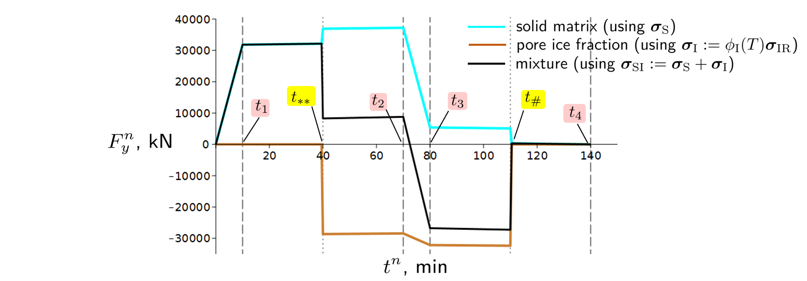
Using both time-loading and time-reaction curves plotted in Figures 1 and 2, respectively, the following is observed:

1. Time interval $(0,t_1)$. The solid matrix is under the constant positive temperature and is experiencing vertical tension. The recovered reaction $F_y$ on $\Gamma_\mathrm{top}$ is linearly growing.

2. Time interval $(t_1,t_2)$. The displacement loading on $\Gamma_\mathrm{top}$ is kept constant, whereas the specimen temperature is decreasing from positive to subzero with $t_{**}:=\frac{1}{2}(t_2-t_1)\in(t_1,t_2)$ being the freezing moment.

   • On sub-interval $(t_1,t_{**})$ the temperature is decreasing from the positive to $T_\mathrm{m}$. The solid matrix contracts yielding the slight increase of the reaction $F_y$ on $\Gamma_\mathrm{top}$, as expected.

   • At $t=t_{\*\*}$, one has $T=T_\mathrm{m}$ such that the Sigmoid ice-fraction indicator function takes the value $\frac{1}{2}$ (both liquid water and ice fractions are present equally). In other words, liquid-to-ice phase change happens in the “small vicinity” of $t_{\*\*}$. Since during such phase transition liquid expands by 9% thus pushing up the fixed top edge, the reaction on $\Gamma_\mathrm{top}$ is expected to drop. It can be seen that the model fulfils such prediction. Also notice that after $t_{**}$, our specimen is already a mixture of a (deformed) solid matrix and an (undeformed) pore ice.

   • On sub-interval $(t_{**},t_2)$, the temperature keeps on decreasing thus causing further contraction of solid matrix and the already formed ice. This results in a slight linear increase of the reaction $F_y$ on $\Gamma_\mathrm{top}$.

3. Time interval $(t_2,t_3)$. The subzero temperature is kept constant, and we start unloading the completely frozen specimen by reducing the vertical displacement loading to its initial (zero) value. Actual unloading applies to the solid matrix, as it was previously deformed (stretched) vertically, whereas the pore ice is experiencing compression. This can be observed by assessing the recovered reaction curves of the corresponding constituents. The total reaction force on $\Gamma_\mathrm{top}$ also decays on this time interval and even enters the negative range. The latter is the indication that the solid-ice mixture remains under compression even when $\bar{u}^n$ on $\Gamma_\mathrm{top}$ reaches $0$. This is expected since for the pore ice this is a deformed configuration.

4. Time interval $(t_3,t_4)$. The vertical displacement on $\Gamma_\mathrm{top}$ is kept at zero level and we start warming the completely frozen specimen. The temperature is increased from negative to the very initial positive value with $t_{\\#}:=\frac{1}{2}(t_4-t_3)\in(t_4,t_3)$ being the melting moment.

   • On sub-interval $(t_3,t_{\\#})$ the specimen expands due to the increase of thermal loading thus pushing upwards the fixed top boundary $\Gamma_\mathrm{top}$. The recovered reaction $F_y$ is hence slightly increasing in negative direction.

   • In the “small vicinity” of melting moment $t_{\\#}$ ice-to-liquid phase transition happens. This is accompanied by 9$\%$ of volume contraction of ice. Since the ice phase ceases to be present, the negative reaction force $F_y$ on $\Gamma_\mathrm{top}$ drops to very small positive value. This value is not zero since a slight contraction of the solid matrix at temperature $T=T_\mathrm{m}$ is still present.

   • On sub-interval $(t_{\\#},t_4)$, further warming of solid matrix goes on till the temperature reaches the very initial positive value. The specimen continues its thermal expansion and finally returns to its initial undeformed state. The reaction $F_y$ returns back to $0$ as well, as expected.

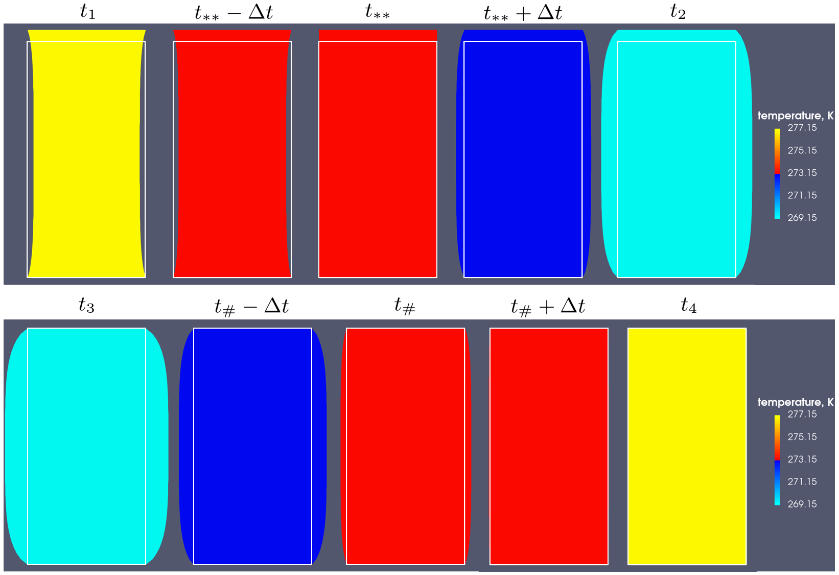
Figure 3 presents snapshots of a specimen’s deformed configuration at the time moments as in Figures 1 and 2. The fill corresponds to specimen’s temperature, and a white frame stands for the undeformed configuration to highlight deformation shape and magnitude. (We notice that in each plots the computed displacement components $u_x$ and $u_y$ have been exaggerated by factors 10 and 80, respectively). The deformation plots supplement and illustrate the above observations and conclusions drawn.

Figure 3: Specimen deformation plots at the corresponding time moments.