Gas Diffusion
![]() This page is based on a Jupyter notebook.
This page is based on a Jupyter notebook.


 |
|---|
1D Linear Diffusion
Analytical Solution
The solution of the diffusion equation for a point x in time t reads:
$ c(x,t) = \left(c_0-c_i\right)\operatorname{erfc}\left(\frac{x}{\sqrt{4Dt}}\right)+c_i$
where $c$ is the concentration of a solute in mol$\cdot$m$^{-3}$, $c_i$ and $c_b$ are initial and boundary concentrations; $D$ is the diffusion coefficient of the solute in water, x and t are location and time of solution.
import os…
(click to toggle)
import os
from pathlib import Path

import matplotlib.pyplot as plt
import numpy as np
import ogstools as ot
import pyvista as pv
from scipy.special import erfc
def Diffusion(x, t):…
(click to toggle)
def Diffusion(x, t):
    "Analytical solution of the diffusion equation"
    d = np.sqrt(4 * D * t)
    return (c_b - c_i) * erfc(
        np.divide(x, d, where=(d != 0), out=np.ones_like(x * d) * 1e6)
    ) + c_i


def concentration(xm_WL):
    "Utility-function transforming mass fraction into conctration"
    xm_CL = 1.0 - xm_WL
return xm_CL / beta_cMaterial properties and problem specification
H = 7.65e-6 # Henry-coefficien…
(click to toggle)
H = 7.65e-6  # Henry-coefficien
beta_c = 2.0e-6  # Compressibility of solution
D = 1.0e-9  # Diffusion coefficient
pGR_b = 9e5  # Boundary gas pressure
pGR_i = 1e5  # Initial gas pressure
c_b = concentration(1.0 - (beta_c * H * pGR_b))  # Boundary concentration
c_i = concentration(1.0 - (beta_c * H * pGR_i)) # Initial concentrationNumerical Solution
out_dir = Path(os.environ.get("OGS_TESTRUNNER_OUT_DIR", "_out"))
out_dir.mkdir(parents=True, exist_ok=True)
model = ot.Project(input_file="diffusion.prj", output_file=f"{out_dir}/modified.prj")…
(click to toggle)
model = ot.Project(input_file="diffusion.prj", output_file=f"{out_dir}/modified.prj")
timestepping = "./time_loop/processes/process/time_stepping"
model.replace_text(1e7, xpath=f"{timestepping}/t_end")
model.replace_text(5e4, xpath=f"{timestepping}/timesteps/pair/delta_t")
model.replace_text(1, xpath="./time_loop/output/timesteps/pair/each_steps")
model.replace_text("XDMF", xpath="./time_loop/output/type")
model.write_input()
model.run_model(logfile=f"{out_dir}/out.txt", args=f"-o {out_dir} -m .")Project file written to output.
Simulation: /var/lib/gitlab-runner/builds/Sbm-BZZt4/1/ogs/build/release-all/Tests/Data/TH2M/H/diffusion/diffusion/modified.prj
Status: finished successfully.
Execution took 12.223031044006348 s
ms = ot.MeshSeries(f"{out_dir}/result_diffusion_domain.xdmf")…
(click to toggle)
ms = ot.MeshSeries(f"{out_dir}/result_diffusion_domain.xdmf")

def plot_results_errors(x: np.ndarray, y: np.ndarray, y_ref: np.ndarray,
         labels: list, x_label: str, colors: list):  # fmt: skip
    "Plot numerical results against analytical solution"
    rel_errors = (np.asarray(y_ref) - np.asarray(y)) / np.asarray(y_ref)
    assert np.all(np.abs(rel_errors) <= 0.3)
    fig, (ax1, ax2) = plt.subplots(1, 2, figsize=(14, 4))

    ax1.set_xlabel(x_label, fontsize=12)
    ax2.set_xlabel(x_label, fontsize=12)
    ax1.set_ylabel("$c$ / mol m$^{-3}$", fontsize=12)
    ax2.set_ylabel(r"$\epsilon_\mathrm{abs}$ / mol m$^{-3}$", fontsize=12)
    for i, rel_error in enumerate(rel_errors):
        ax1.plot(x, y[i], "--", lw=2, label=labels[i], c=colors[i])
        ax1.plot(x, y_ref[i], "-", lw=1, c=colors[i])
        ax2.plot(x, rel_error, "-", lw=2, label=labels[i], c=colors[i])
    ax1.plot([], [], "--k", label="OGS-TH2M")
    ax1.plot([], [], "-k", label="analytical")
    ax1.legend(loc="right")
    ax2.legend(loc="right")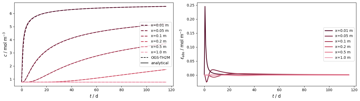
fig.tight_layout()Concentration vs. time at different locations
obs_pts = np.asarray([(x, 0, 0) for x in [0.01, 0.05, 0.1, 0.2, 0.5, 1.0]])…
(click to toggle)
obs_pts = np.asarray([(x, 0, 0) for x in [0.01, 0.05, 0.1, 0.2, 0.5, 1.0]])
num_values = concentration(ms.probe(obs_pts, "xmWL").T)
ref_values = [Diffusion(x, ms.timevalues) for x in obs_pts[:, 0]]
leg_labels = [f"x={pt[0]} m" for pt in obs_pts]
reds = ["#4a001e", "#731331", "#9f2945", "#cc415a", "#e06e85", "#ed9ab0"]
time = ms.timevalues / 3600 / 24
plot_results_errors(time, num_values, ref_values, leg_labels, "$t$ / d", reds)
Concentration vs. location at different times
timevalues = np.asarray([1e6, 2e6, 4e6, 6e6, 8e6, 1e7])…
(click to toggle)
timevalues = np.asarray([1e6, 2e6, 4e6, 6e6, 8e6, 1e7])
timesteps = [ms.closest_timestep(tv) for tv in timevalues]
xs = np.linspace(0, 0.4, 40)
line = pv.PointSet([(x, 0, 0) for x in xs])
num_values = [concentration(line.sample(ms[ts])["xmWL"]) for ts in timesteps]
ref_values = [Diffusion(xs, tv) for tv in timevalues]
leg_labels = [f"{tv:.0e} s" for tv in timevalues]
blues = ["#0b194c", "#163670", "#265191", "#2f74b3", "#5d94cb", "#92b2de"]
plot_results_errors(xs, num_values, ref_values, leg_labels, "$x$ / m", blues)
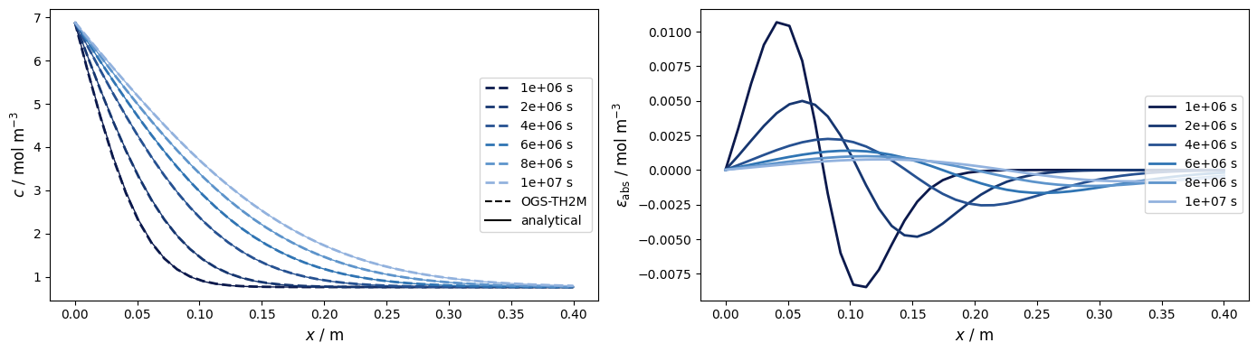
The numerical approximation approaches the exact solution quite well. Deviations can be reduced if the resolution of the temporal discretisation is increased.
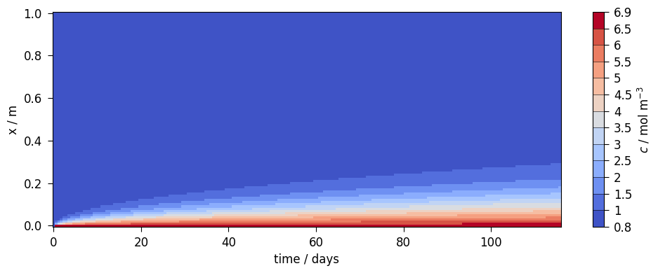
Concentration over time and space
pts = np.linspace([0.0, 0.0, 0.0], [0.3, 0.0, 0.0], 500)…
(click to toggle)
pts = np.linspace([0.0, 0.0, 0.0], [0.3, 0.0, 0.0], 500)
var = ot.variables.Scalar("xmWL", func=concentration)
ot.plot.setup.time_unit = "days"
fig = ms.scale(time=("s", "days")).plot_time_slice(
    "time", "x", var, figsize=[10, 4], fontsize=12
)
fig.axes[1].set_ylabel("$c$ / mol m$^{-3}$")
fig.tight_layout()/var/lib/gitlab-runner/builds/Sbm-BZZt4/1/ogs/build/release-all/.venv/lib/python3.13/site-packages/ogstools/meshlib/mesh_series.py:910: UserWarning: The input coordinates to pcolormesh are interpreted as cell centers, but are not monotonically increasing or decreasing. This may lead to incorrectly calculated cell edges, in which case, please supply explicit cell edges to pcolormesh.
ax.pcolormesh(x_vals, y_vals, values, cmap=cmap, norm=norm)
This article was written by Norbert Grunwald. If you are missing something or you find an error please let us know.
Generated with Hugo 0.147.9
in CI job 683680
|
Last revision: October 19, 2022