H2M Liakopoulos benchmark
![]() This page is based on a Jupyter notebook.
This page is based on a Jupyter notebook.


import os…
(click to toggle)
import os
from pathlib import Path

import matplotlib.pyplot as plt
import numpy as np
import ogstools as ot

out_dir = Path(os.environ.get("OGS_TESTRUNNER_OUT_DIR", "_out"))
if not out_dir.exists():
out_dir.mkdir(parents=True)H2M process: Liakopoulos benchmark
Problem description

The Liakopoulos experiment was dealing with a sand column which was filled with water first and then drained under gravity. A sketch of the related model set-up including initial and boundary conditions is shown in the above figure. A detailed description of the underlying OGS model is given in Grunwald et al. (2022). Two hydraulic models have been compared; two-phase flow with a mobile and a Richards flow with an immobile gas phase coupled to mechanical processes. Due to the absence of analytical solutions various numerical solutions have been compared in the past (see Grunwald et al., 2022).
The model parameters are given in the below table.
| Parameter | Value | Unit |
|---|---|---|
| Permeability | $k^0_\textrm{S}$ = 4.5 $\times$ 10$^{-13}$ | m$^2$ |
| Porosity | $\phi$ = 0.2975 | - |
| Young’s modulus | $E$ = 1.3 | MPa |
| Poisson ratio | $\nu$ = 0.4 | - |
| Dynamic viscosity of gas phase | $\mu_\textrm{GR}$ = 1.8 $\times$ 10$^{-5}$ | Pa s |
| Dynamic viscosity of liquid phase | $\mu_\textrm{LR}$ = 1.0 $\times$ 10$^{-3}$ | Pa s |
| Density of liquid phase | $\rho_\textrm{LR}$ = 1.0$\times$ 10$^3$ | kg m$^{-3}$ |
| Density of solid phase | $\rho_\textrm{SR}$ = 2.0$\times$ 10$^3$ | kg m$^{-3}$ |
Numerical solution
prj_file = "liakopoulos_TH2M.prj"…
(click to toggle)
prj_file = "liakopoulos_TH2M.prj"
model = ot.Project(input_file=prj_file, output_file=prj_file)
model.run_model(logfile=f"{out_dir}/out.txt", args=f"-o {out_dir}")Project file written to output.
Simulation: liakopoulos_TH2M.prj
Status: finished successfully.
Execution took 7.222959041595459 s
ms = ot.MeshSeries(f"{out_dir}/result_liakopoulos.pvd")…
(click to toggle)
ms = ot.MeshSeries(f"{out_dir}/result_liakopoulos.pvd")

# plausibility checks
max_vals = {"gas_pressure": 1.02e5, "capillary_pressure": 1e4,
            "saturation": 1.0001, "displacement": 0.005}  # fmt:skip


def plot_sample(var: ot.variables.Scalar) -> None:
    fig, ax = plt.subplots(figsize=[6, 3], dpi=150)
    ax.set_xlabel(r"$y$ / m")
    ax.set_ylabel(var.get_label())
    for mesh, t in zip(ms, ms.timevalues):
        line_mesh = mesh.sample_over_line([0, 0, 0], [0, 1, 0])
        vals = line_mesh.sample(mesh)[var.data_name]
        assert np.all(np.abs(vals) <= max_vals[var.data_name]), max(abs(vals))
        ax.plot(line_mesh.points[:, 1], var.transform(vals), label=f"{t=}", lw=2.5)
    ax.legend()
    ax.grid()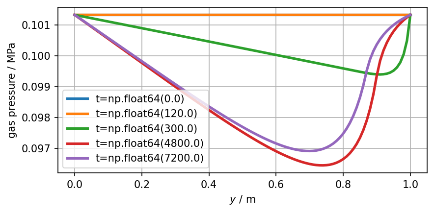
fig.tight_layout()Gas Pressure
plot_sample(ot.variables.Scalar("gas_pressure", "Pa", "MPa"))
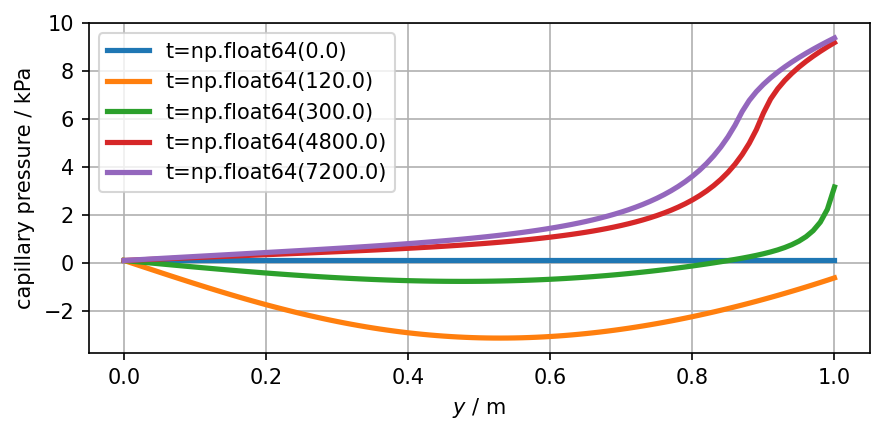
Capillary Pressure
plot_sample(ot.variables.Scalar("capillary_pressure", "Pa", "kPa"))
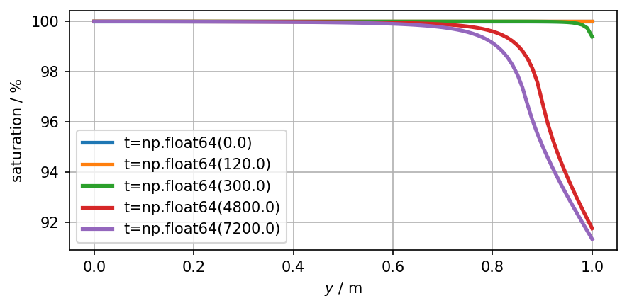
Saturation
plot_sample(ot.variables.Scalar("saturation", "", "%"))
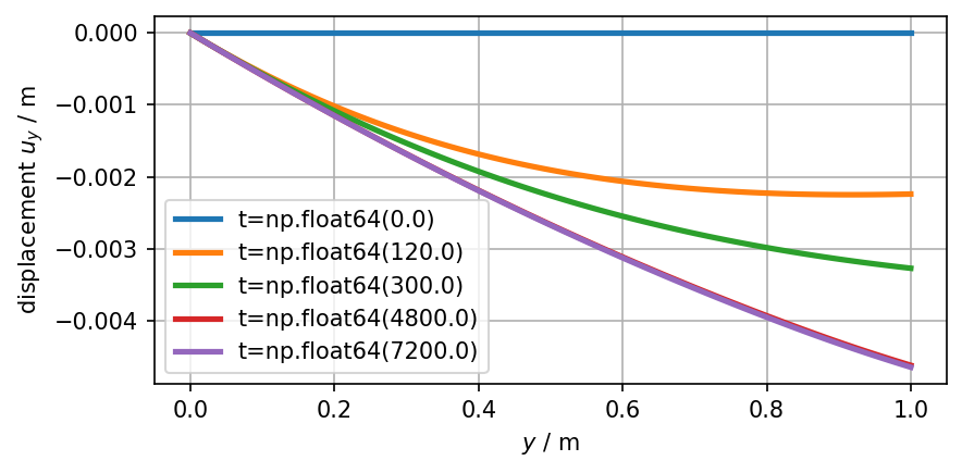
Vertical Displacement
plot_sample(ot.variables.displacement["y"])
OGS links
- description: https://www.opengeosys.org/docs/benchmarks/
- project file: https://gitlab.opengeosys.org/ogs/ogs/-/blob/master/Tests/Data/TH2M/H2M/Liakopoulos/liakopoulos_TH2M.prj
Credits
- Norbert Grunwald for set-up the OGS benchmark, https://gitlab.opengeosys.org/ogs/ogs/-/blob/master/Tests/Data/TH2M/H2M/Liakopoulos/liakopoulos_TH2M.prj
References
Grunwald, N., Lehmann, C., Maßmann, J., Naumov, D., Kolditz, O., Nagel, T., (2022): Non-isothermal two-phase flow in deformable porous media: systematic open-source implementation and verification procedure. Geomech. Geophys. Geo-Energy Geo-Resour. 8 (3), art. 107 https://doi.org/10.1007/s40948-022-00394-2
Kolditz, O., Görke, U.-J., Shao, H., Wang, W., (eds., 2012): Thermo-hydro-mechanical-chemical processes in porous media: Benchmarks and examples. Lecture Notes in Computational Science and Engineering 86, Springer, Berlin, Heidelberg, 391 pp https://link.springer.com/book/10.1007/978-3-642-27177-9
Lewis RW, Schrefler BA (1998): The finite element method in the static and dynamic deformation and consolidation of porous media. Wiley, New York https://www.wiley.com/en-us/The+Finite+Element+Method+in+the+Static+and+Dynamic+Deformation+and+Consolidation+of+Porous+Media%2C+2nd+Edition-p-9780471928096
Liakopoulos AC (1964): Transient flow through unsaturated porous media. PhD thesis. University of California, Berkeley, USA. sources: OGS BMB1 (sec. 13.2
This article was written by Norbert Grunwald, Olaf Kolditz. If you are missing something or you find an error please let us know.
Generated with Hugo 0.147.9
in CI job 576931
|
Last revision: August 16, 2022