LargeDeformations: Torsion of a hyperelastic bar

This page is based on a Jupyter notebook.

Convergence under large deformations (preliminary)

In this benchmark we impose large tensile and torsional deformations on a hyperelastic prismatic bar. The material model is a Saint-Venant-Kirchhoff material law for initial testing.

import os… (click to toggle)

import os
from pathlib import Path

import matplotlib.pyplot as plt
import numpy as np
import ogstools as ot
import pandas as pd
import pyvista as pv
from ogstools import logparser

pv.set_jupyter_backend("static" if "CI" in os.environ else "client")… (click to toggle)

pv.set_jupyter_backend("static" if "CI" in os.environ else "client")

out_dir = Path(os.environ.get("OGS_TESTRUNNER_OUT_DIR", "_out"))
out_dir.mkdir(parents=True, exist_ok=True)

model = ot.Project(input_file="bar1to6_torsion.prj", output_file="bar1to6_torsion.prj")… (click to toggle)

model = ot.Project(input_file="bar1to6_torsion.prj", output_file="bar1to6_torsion.prj")
model.run_model(logfile=out_dir / "out.txt", args=f"-o {out_dir}")
mesh = ot.MeshSeries(out_dir / "bar1to6_torsion.pvd")[-1]

Project file written to output.
Simulation: bar1to6_torsion.prj
Status: finished successfully.
Execution took 5.088003396987915 s

Boundary conditions

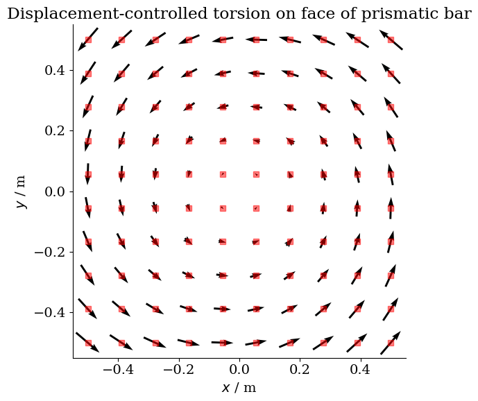
The bar of dimensions $1 \times 1 \times 6$ m³ is stretched by $\lambda = 1.5$ in the axial direction and twisted by 180°. The following graph illustrates the torsion bc.

top_pts = mesh.points[:, 2] == mesh.bounds[5]… (click to toggle)

top_pts = mesh.points[:, 2] == mesh.bounds[5]
top_surf = mesh.extract_points(top_pts, False, False).delaunay_2d()
fig = ot.plot.contourf(top_surf, ot.variables.displacement, figsize=(8, 6), fontsize=14)

png

Let’s plot the result.

pl = pv.Plotter()… (click to toggle)

pl = pv.Plotter()
pl.camera_position = (-0.5, -0.5, 0.4)
pl.add_mesh(mesh, color="lightgrey", style="wireframe", line_width=1)
deformed_mesh = mesh.warp_by_vector("displacement")
pl.add_mesh(deformed_mesh, scalars="displacement", show_edges=True, cmap="jet")
pl.show_axes()
pl.reset_camera()
pl.show()

[0m[33m2025-09-09 17:44:23.935 (   7.380s) [    70E2C6663B80]vtkXOpenGLRenderWindow.:1416  WARN| bad X server connection. DISPLAY=[0m

png

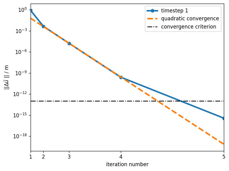
Convergence

What we’re more interested in, is the convergence behaviour over time. The large deformations were applied in only 5 load steps to challenge the algorithm.

log_file_raw = logparser.parse_file(f"{out_dir}/out.txt")… (click to toggle)

log_file_raw = logparser.parse_file(f"{out_dir}/out.txt")
log_df = pd.DataFrame(log_file_raw)
for ts in range(1, 6):
    dxs = log_df[log_df["time_step"] == ts]["dx"].dropna().to_numpy()
    slopes = np.log10(dxs)[1:] / np.log10(dxs)[:-1]
    # not checking slope of last ts (below quadratic due to precision limit)
    assert np.all(slopes[:-1] > 1.9)

fig, ax = plt.subplots(dpi=120)… (click to toggle)

fig, ax = plt.subplots(dpi=120)
ts1_df = log_df[log_df["time_step"] == 1]
its, dxs = ts1_df[["iteration_number", "dx"]].dropna().to_numpy(float).T
ax.plot(its, dxs, "-o", label="timestep 1", lw=3)

offset = 3 - np.log2(-np.log10(dxs[2]))  # to touch the data at dx(it=3)
quad_slope = 10 ** -(2 ** (its - offset))
ax.plot(its, quad_slope, "--C1", lw=3, label="quadratic convergence")

ax.axhline(1e-13, ls="-.", color="k", label="convergence criterion")
ax.set_xscale("function", functions=(lambda x: 2**x, lambda x: np.log10(x - 2)))
ax.set_yscale("log")
ax.set_xlim([1, 5])
ax.set_xticks(its)
ax.set_xlabel("iteration number")
ax.set_ylabel("$|| \\Delta \\vec{u}$ || / m")
ax.legend()
fig.tight_layout()

png

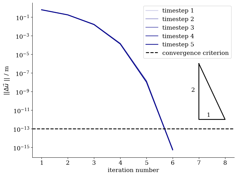
We observe quadratic convergence in the proximity of the solution supporting the implementation of the geometric stiffness matrix. The last iteration converges slightly less then quadratic since we reach the numerical precision limit at this point.

This article was written by Thomas Nagel. If you are missing something or you find an error please let us know.
Generated with Hugo 0.147.9 in CI job 608965 | Last revision: March 2, 2023