This page is based on a Jupyter notebook.

Introduction

This tutorial describes the implementation in OGS for a method for mimicking the behavior of a moving Dirichlet boundary condition, applicable to HeatConduction processes. Moving Dirichlet boundary conditions are useful, for example, to emulate the rise during construction of a thermally active structure, e.g., a landfill embankment or a sulfide tailings dam.

Context

This method derives from a project aimed at studying heat generation and transport in a major thermally-active landfill in Colombia which stores municipal solid waste with high (>60%) organic content. In these systems, the sequential rise of the landfill embankment during construction generates moving boundary conditions that must be accounted for in modeling.

In order to simulate heat generation due to biodegradation of the waste organic fraction, a time- and temperature-dependent heat generation function (Hanson et al., 2013) was implemented in the model with units W/m³ using a Python source term:

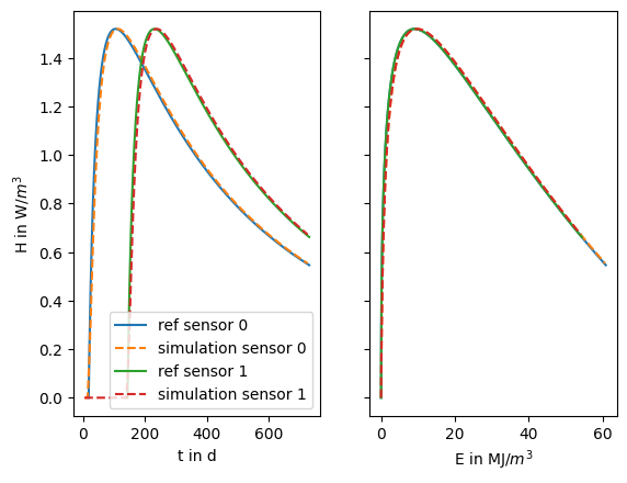
$$ H \;=\; F A \left(\frac{t}{B + t}\right) \left(\frac{C}{C + t}\right) e^{-\sqrt{\frac{t}{D}}}. $$

where $F$ is a temperature-dependent factor that ranges from 0.0 to 1.0 and represents a dual-ramped scaling function (Hanson et al., 2013), $H$ is the heat generation rate (units W/m³), $t$ is time (seconds), $A$ is the peak heat generation rate factor (units W/m³), $B$ and $C$ are shape factors (seconds), and $D$ is the decay rate factor (seconds). In the Python source term, the heat generation is also formulated in the energy expended domain (units: MJ/m³) to account for the system’s energy consumption.

A moving Dirichlet boundary condition is required in this problem to represent the onset of heat generation after each waste layer is constructed, while avoiding heat loss to the free domain.

Implementation in OGS

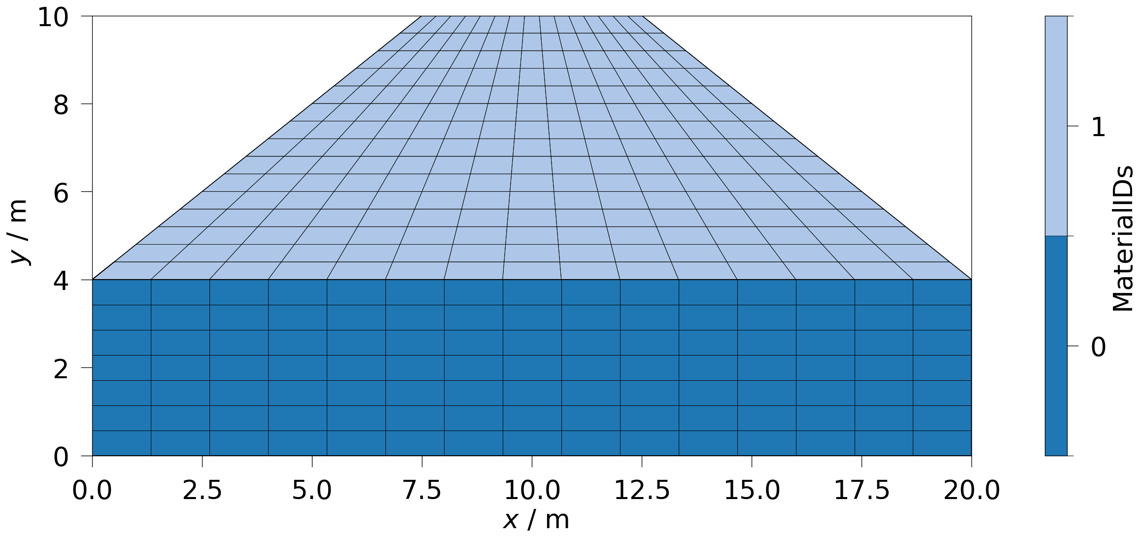
A simple two-dimensional, two-layer model was created to illustrate the implementation of the moving Dirichlet boundary condition. The bottom layer (4 m thick) represents the geological subsoil on which the landfill is constructed. The top trapezoidal layer (6 m high) represents the final simplified geometry of a landfill. The model was meshed in Gmsh using a structured mesh (330 cells, 368 nodes).

import os… (click to toggle)

import os
from pathlib import Path

import gmsh
import matplotlib.pyplot as plt
import numpy as np
import ogstools as ot
import pandas as pd
from scipy.integrate import cumulative_trapezoid

out_dir = Path(os.environ.get("OGS_TESTRUNNER_OUT_DIR", "_out"))
out_dir.mkdir(parents=True, exist_ok=True)

# Mesh the landfill and subsurface body… (click to toggle)

# Mesh the landfill and subsurface body
gmsh.initialize()
gmsh.model.add("simple_model")

p0 = gmsh.model.occ.addPoint(0, 0, 0)
p1 = gmsh.model.occ.addPoint(0, 4, 0)
p2 = gmsh.model.occ.addPoint(20, 4, 0)
p3 = gmsh.model.occ.addPoint(20, 0, 0)
p4 = gmsh.model.occ.addPoint(7.5, 10, 0)
p5 = gmsh.model.occ.addPoint(12.5, 10, 0)

gmsh.model.occ.synchronize()

l0 = gmsh.model.occ.addLine(p0, p1)
l1 = gmsh.model.occ.addLine(p1, p2)
l2 = gmsh.model.occ.addLine(p2, p3)
l3 = gmsh.model.occ.addLine(p3, p0)
l4 = gmsh.model.occ.addLine(p1, p4)
l5 = gmsh.model.occ.addLine(p4, p5)
l6 = gmsh.model.occ.addLine(p5, p2)

gmsh.model.occ.synchronize()

bottom_curve = gmsh.model.occ.addCurveLoop([l0, l1, l2, l3])
top_curve = gmsh.model.occ.addCurveLoop([l4, l5, l6, l1])

gmsh.model.occ.synchronize()

bottom_domain = gmsh.model.occ.addPlaneSurface([bottom_curve])
top_domain = gmsh.model.occ.addPlaneSurface([top_curve])

gmsh.model.occ.synchronize()

gmsh.model.addPhysicalGroup(dim=2, tags=[bottom_domain], name="bottom_domain")
gmsh.model.addPhysicalGroup(dim=2, tags=[top_domain], name="top_domain")
gmsh.model.addPhysicalGroup(dim=1, tags=[l4, l5, l6], name="top_lines")

gmsh.model.occ.synchronize()

gmsh.model.mesh.setTransfiniteCurve(l1, 16)
gmsh.model.mesh.setTransfiniteCurve(l3, 16)
gmsh.model.mesh.setTransfiniteCurve(l5, 16)

gmsh.model.mesh.setTransfiniteCurve(l0, 8)
gmsh.model.mesh.setTransfiniteCurve(l2, 8)

gmsh.model.mesh.setTransfiniteCurve(l4, 16)
gmsh.model.mesh.setTransfiniteCurve(l6, 16)
gmsh.model.mesh.setTransfiniteSurface(bottom_domain)
gmsh.model.mesh.setTransfiniteSurface(top_domain)
gmsh.model.mesh.setRecombine(2, top_domain)
gmsh.model.mesh.setRecombine(2, bottom_domain)
gmsh.model.mesh.generate(2)

mesh_name = "simple_model"
msh_file = f"{out_dir}/{mesh_name}.msh"
gmsh.write(msh_file)
gmsh.finalize()


meshes = ot.Meshes.from_gmsh(msh_file, log=False, dim=[2])

Info    : Meshing 1D...
Info    : [  0%] Meshing curve 1 (Line)
Info    : [ 20%] Meshing curve 2 (Line)
Info    : [ 30%] Meshing curve 3 (Line)
Info    : [ 50%] Meshing curve 4 (Line)
Info    : [ 60%] Meshing curve 5 (Line)
Info    : [ 80%] Meshing curve 6 (Line)
Info    : [ 90%] Meshing curve 7 (Line)
Info    : Done meshing 1D (Wall 0.000355544s, CPU 0.000545s)
Info    : Meshing 2D...
Info    : [  0%] Meshing surface 1 (Transfinite)
Info    : [ 60%] Meshing surface 2 (Transfinite)
Info    : Done meshing 2D (Wall 0.000323536s, CPU 0.000407s)
Info    : 368 nodes 425 elements
Info    : Writing '/var/lib/gitlab-runner/builds/K-X1vcp78/0/ogs/build/release-all/web/content/docs/tutorials/moving_bc/notebook-moving_bc/simple_model.msh'...
Info    : Done writing '/var/lib/gitlab-runner/builds/K-X1vcp78/0/ogs/build/release-all/web/content/docs/tutorials/moving_bc/notebook-moving_bc/simple_model.msh'

# Visualize the mesh (MaterialID 0: subsurface 1: landfill body)… (click to toggle)

# Visualize the mesh (MaterialID 0: subsurface 1: landfill body)
fig = ot.plot.contourf(
    meshes.domain, variable=ot.variables.material_id, interactive=False
)
fig.show()

The moving Dirichlet boundary condition (in the positive y direction) was mimicked as follows:

Define values for the thermal properties of the landfill body (i.e., specific_heat_capacity = 2276 J/kg.K and thermal_conductivity = 1.15 W/m.K for this example) at the integration points of the elements already constructed inside the landfill embankment domain.
Assign a very high (“infinite”) value (1e12 in this example) to the specific_heat_capacity of the landfill body at the integration points of the elements not yet constructed inside the landfill embankment. A material with “infinite” specific_heat_capacity is physically expected to absorb all the produced heat. Note that it is not recommended to assign an infinite value to the thermal_conductivity of the landfill body because misleading results have been observed due to strong coupling related to very high values of the conductance matrix during the simulations.
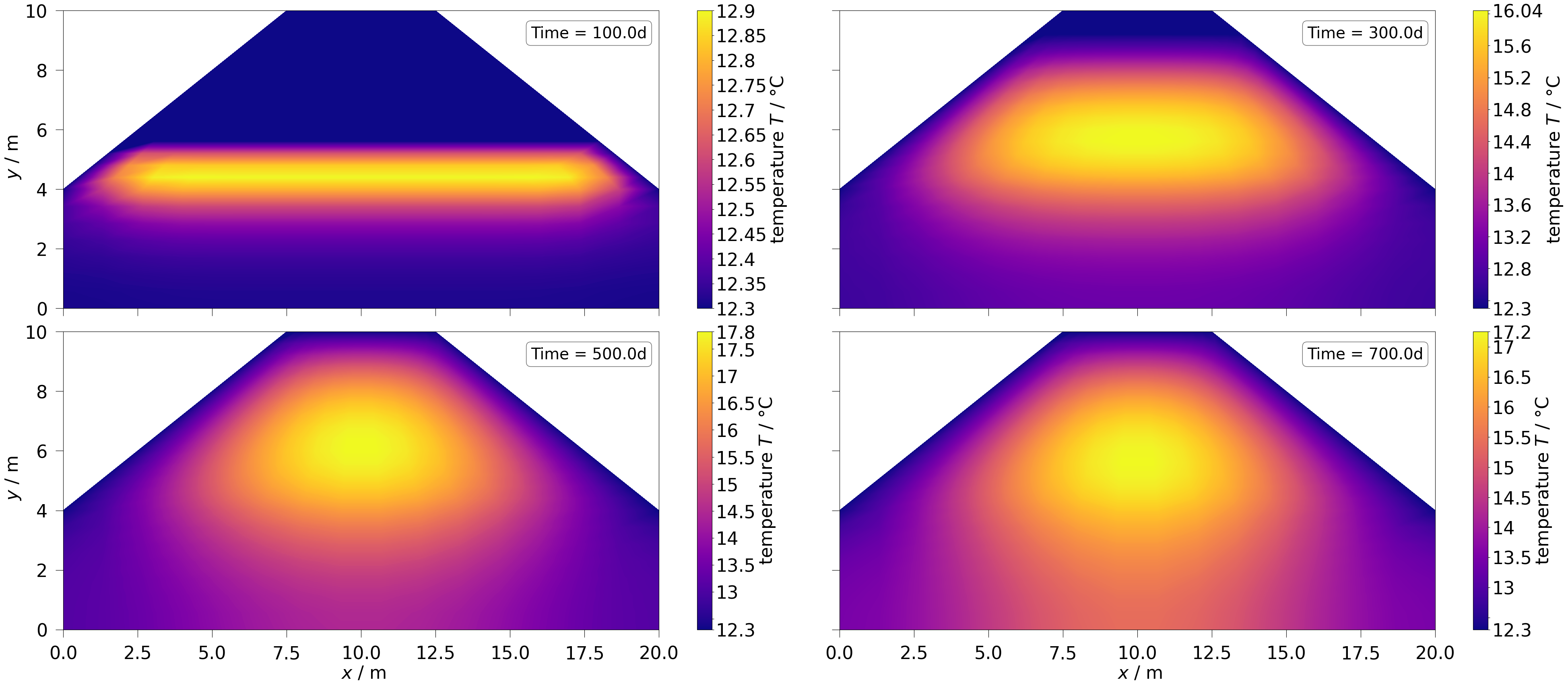
In the .prj file include an <expression> function consisting of an if clause for the y coordinate where if y is greater than (>) a given moving geometric boundary, the thermal properties are set to “infinite”; otherwise, they are set to the desired physical values. The value against which y is compared is a time-dependent moving geometric boundary, which corresponds to the rate of vertical construction of the landfill embankment (in this example 2e-7 m/s, i.e., about 6.3 m/year).

        <medium id="1">
        <!-- Landfill waste -->
            <phases/>
            <properties>
                <property>
                    <name>specific_heat_capacity</name>
                    <type>Function</type>
                    <value>
                        <expression>if(y &gt; 4 + t * 2e-7, 1e12, 2276)</expression>
                        <!-- Construction started at 4m, Construction rate: about 6.3 m/yr (2e-7 m/s) -->
                    </value>
                </property>
                <property>
                    <name>thermal_conductivity</name>
                    <type>Constant</type>
                    <value>1.15</value>
                </property>
                <property>
                    <name>density</name>
                    <type>Constant</type>
                    <value>999</value>
                </property>
            </properties>
        </medium>

# execute the model… (click to toggle)

# execute the model
prj = ot.Project(input_file="landfill.prj")

model = ot.Model(project=prj, meshes=meshes)
sim = model.run()

results = sim.meshseries… (click to toggle)

results = sim.meshseries

# 4 timeframes figure
variable = ot.variables.temperature
fig, axs = plt.subplots(2, 2, figsize=(40, 17), sharex=True, sharey=True)
plot_timesteps = [20, 60, 100, 140]

bbox = {
    "boxstyle": "round,pad=0.3",
    "facecolor": "white",
    "edgecolor": "black",
    "alpha": 0.6,
}

for i, timestep in enumerate(plot_timesteps):
    ax = axs[int(i / 2)][int(i % 2)]
    ot.plot.contourf(
        results.mesh(timestep), variable, fig=fig, ax=ax, continuous_cmap=True
    )

    ax.text(
        0.98,
        0.95,
        f"Time = {results.timevalues[timestep]/(24*3600)}d",
        transform=ax.transAxes,
        fontsize=28,
        ha="right",
        va="top",
        bbox=bbox,
    )

fig.tight_layout()
fig.show()

# Plot the temperature over time at observation points in the landfill body… (click to toggle)

# Plot the temperature over time at observation points in the landfill body
probe_ms = results.probe(points=[(10.0, y, 0.0) for y in [4.0, 6.0, 8.0]])
fig = ot.plot.line(
    probe_ms,
    var1="time",
    var2=ot.variables.temperature,
    labels=["y=4.0m", "y=6.0m", "y=8.0m"],
)
fig.show()

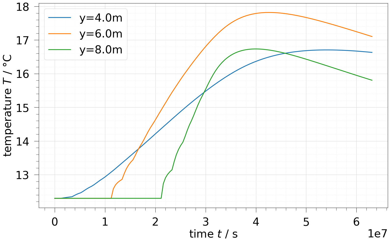
It can be seen that the implementation simulates the sequential rise of the Dirichlet boundary condition during heat generation in the landfill, which is consistent with the practical growth of the facility embankment during construction.

# Define semi-empirical time-dependent logarithmic growth and decay formulation for the heat generation (Hanson et al., 2022)

… (click to toggle)

# Define semi-empirical time-dependent logarithmic growth and decay formulation for the heat generation (Hanson et al., 2022)

# Constants to control the shape of the heat generation function
A = 4.88  # peak heat generation in W/m³
B = 50 * 24 * 60 * 60  # shape constant for the peak heat generation in seconds
C = 5000 * 24 * 60 * 60  # shape constant for the peak heat generation in seconds
D = 180 * 24 * 60 * 60  # decay rate factor in seconds


def time_dependent_source(t):
    return A * ((t / (B + t)) * (C / (C + t))) * np.exp(-np.sqrt(t / D))


# Calculate heat generation as a function of expended-energy (Hanson et al. 2013)


def energy_expended(t):
    source_values = time_dependent_source(t)
    energy_vals = cumulative_trapezoid(source_values, t, initial=0)
    return energy_vals, source_values


# calculate the time, at which the construction starts in dependence to the y-coordinate


def time_of_construction(y):
    return (y - 4) / 2e-7

# Read the heat generation and energy expended results from sensor csv-files written in the source_term.py… (click to toggle)

# Read the heat generation and energy expended results from sensor csv-files written in the source_term.py
sensor_coords_list = [
    (10.369722119417698, 4.315470053837926, 0.0),
    (10.26536317669089, 6.484529946162075, 0.0),
]

sensor_0 = pd.read_csv(out_dir / "energy_expended_sensor_index_0.csv")
sensor_1 = pd.read_csv(out_dir / "energy_expended_sensor_index_1.csv")

sensor_0_t_construction = time_of_construction(sensor_coords_list[0][1])
sensor_1_t_construction = time_of_construction(sensor_coords_list[1][1])
timevalues_sensor_0 = np.linspace(
    sensor_0_t_construction, 2 * 365 * 24 * 3600, 2 * 365 * 24
)
timevalues_sensor_1 = np.linspace(
    sensor_1_t_construction, 2 * 365 * 24 * 3600, 2 * 365 * 24
)

# Check the results… (click to toggle)

# Check the results
assert np.allclose(
    time_dependent_source(timevalues_sensor_0 - sensor_0_t_construction),
    np.interp(
        timevalues_sensor_0, sensor_0["time_s"], sensor_0["heat_generation_W/m3"]
    ),
    atol=0.2,
)
assert np.allclose(
    time_dependent_source(timevalues_sensor_1 - sensor_1_t_construction),
    np.interp(
        timevalues_sensor_1, sensor_1["time_s"], sensor_1["heat_generation_W/m3"]
    ),
    atol=0.2,
)

sensor_0_E_exp, sensor_0_source = energy_expended(
    timevalues_sensor_0 - sensor_0_t_construction
)
sensor_1_E_exp, sensor_1_source = energy_expended(
    timevalues_sensor_1 - sensor_1_t_construction
)
assert np.allclose(
    sensor_0["heat_generation_W/m3"],
    np.interp(
        sensor_0["energy_expended_MJ/m3"], sensor_0_E_exp * 1e-6, sensor_0_source
    ),
    atol=0.25,
)
assert np.allclose(
    sensor_1["heat_generation_W/m3"],
    np.interp(
        sensor_1["energy_expended_MJ/m3"], sensor_1_E_exp * 1e-6, sensor_1_source
    ),
    atol=0.25,
)

fig, axs = plt.subplots(1, 2, sharey=True)

axs[0].plot(
    timevalues_sensor_0 / (24 * 3600),
    time_dependent_source(timevalues_sensor_0 - sensor_0_t_construction),
    label="ref sensor 0",
)
axs[0].plot(
    sensor_0["time_s"] / (24 * 3600),
    sensor_0["heat_generation_W/m3"],
    label="simulation sensor 0",
    linestyle="dashed",
)
axs[0].plot(
    timevalues_sensor_1 / (24 * 3600),
    time_dependent_source(timevalues_sensor_1 - sensor_1_t_construction),
    label="ref sensor 1",
)
axs[0].plot(
    sensor_1["time_s"] / (24 * 3600),
    sensor_1["heat_generation_W/m3"],
    label="simulation sensor 1",
    linestyle="dashed",
)
axs[0].set_xlabel("t in d")
axs[0].set_ylabel(r"H in W/$m^3$")

axs[1].plot(sensor_0_E_exp * 1e-6, sensor_0_source, label="ref sensor 0")
axs[1].plot(
    sensor_0["energy_expended_MJ/m3"],
    sensor_0["heat_generation_W/m3"],
    label="simulation sensor 0",
    linestyle="dashed",
)
axs[1].plot(sensor_1_E_exp * 1e-6, sensor_1_source, label="ref sensor 1")
axs[1].plot(
    sensor_1["energy_expended_MJ/m3"],
    sensor_1["heat_generation_W/m3"],
    label="simulation sensor 1",
    linestyle="dashed",
)
axs[1].set_xlabel(r"E in MJ/$m^3$")

axs[0].legend()
fig.show()

References

Hanson, J.L., Yesiller, N., Onnen, M.T., Liu, W.-L., Oettle, N.K., Marinos, J.A.: Development of numerical model for predicting heat generation and temperatures in MSW landfills. Waste Management 33(10), 1993–2000 (2013) https://doi.org/10.1016/j.wasman.2013.04.003

Hanson, J.L., Onnen, M.T., Yesiller, N., Kopp, K.B.: Heat energy potential of municipal solid waste landfills: Review of heat generation and assessment of vertical extraction systems. Renewable and Sustainable Energy Reviews 167, 112835 (2022) https://doi.org/10.1016/j.rser.2022.112835

This article was written by Max Jäschke and Joan Larrahondo. If you are missing something or you find an error please reach out to us on our forum.
Generated with Hugo 0.164.0 in CI job 825193 | Last revision: June 7, 2025

Mimicking a moving Dirichlet Boundary Condition

Introduction

Context

Implementation in OGS

References