Heterogeneous Saturated Mass Transport
- Parabolic/ComponentTransport/heterogeneous/ogs5_H_2D/ogs5_H_2d.prj
- Parabolic/ComponentTransport/heterogeneous/ogs5_H_3D/ogs5_H_3d.prj
Overview
This example involves the usage of a cell-based heterogeneous parameterization for the parameter “intrinsic permeability”. We show a 2D and a 3D setup and compared the results to those from OGS-5; the original examples are described in chapter “5.2 Groundwater flow in a heterogeneous medium” in Kolditz et al. (2012).
We extended the setup to show mass transport in the heterogeneous medium for testing.
Problem description
The setups are steady-state for flow, with an extent of a $100$ m x $100$ m horizontal plane for the 2D setup and a $100$ m x $100$ m x $50$ m cube for the 3D setup. Mesh elements have side lengths of $1$ m. The initial conditions are hydrostatic and concentration $c=0$. The boundary conditions are translated into equivalent hydrostatic pressure values from hydraulic heads $h_{left}=10$ m and $h_{right}=9$ m and for concentration $c_{left}=1$, $c_{right}=0$ for left and right sides, respectively. All other sides are defined as no-flow (Zero-Neumann).
Porosity is $0.01$, specific storage is $0$, fluid density is $1000$ kg$\cdot$m$^{-3}$, dynamic viscosity is $10^{-3}$ Pa$\cdot$s, molecular diffusion coefficient is $2\cdot 10^{-9}$ m$^2\cdot$s$^{-1}$, dispersivities are longitudinal $1$ m and transverse $0.1$ m. The heterogeneous parameter fields of intrinsic permeability are shown in the figures below; creation of the tensor field is documented here .
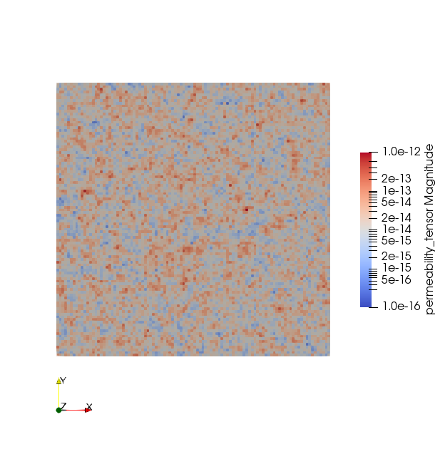
Magnitude of isotropic permeability tensor for 2D setup.
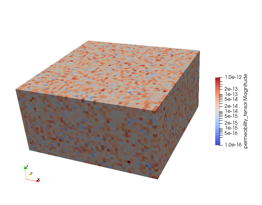
Magnitude of isotropic permeability tensor for 3D setup.
Model results
The comparison of velocity and hydraulic head are shown below. The numerical results of OGS-6 fit very well to the OGS-5 results with relative differences for velocity in the order of ca $10^{-2}$ and for hydraulic head in $10^{-4}$.
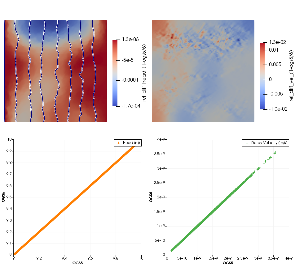
Relative differences of 2D simulation results between OGS-5 and OGS-6. On the top left figure, white lines represent hydraulic head values of OGS-5, blue lines of OGS-6.
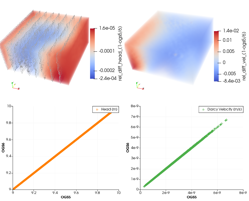
Relative differences of 3D simulation results between OGS-5 and OGS-6. On the top left figure, grey dots represent hydraulic head values of OGS-6.
The mass transport simulation results (figures below) show an expected heterogeneous mass front moving through the domain.
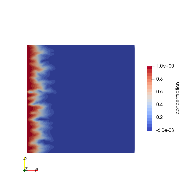
Concentration distribution at simulation time $1e8$ s for the 2D setup.
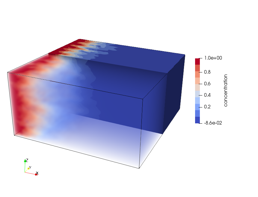
Concentration distribution at simulation time $1e8$ s for the 3D setup.
Literature
Kolditz, O., Görke, U.-J., Shao, H., Wang, W., 2012. Thermo-Hydro-Mechanical-Chemical Processes in Porous Media: Benchmarks and Examples, Lecture notes in computational science and engineering. Springer. ISBN: 3642271766.
 Community Discussion
The following comments are pulled in from our Discourse forum and contain community-generated content.
This article was written by Marc Walther. If you are missing something or you find an error please reach out
to us on our forum.
Generated with Hugo 0.164.0
in CI job 825193
|
Last revision: April 20, 2026
Commit: refactor(MeshLib): remove PropertyVector::push_back 870422dde
| Edit this page on