Heating of a homogeneous volume

This page is based on a Jupyter notebook.

This example is one of the mini-benchmarks of FE-Modelling Task Force (by Andrés Alcolea et. al.). The example is aimed to simulate the coupled THM processes in a fully water saturated unit cubic porous medium ($[0, 1])³$ m$³$) with a linear homogeneous temperature increment from 20$^\circ$C to 30$^\circ$C in 100 days.

The gravity is not considered in all balance equations. Since the temperature is homogeneous, the specific heat capacity is set to zero and thermal conductivity can be any non-zero number. The liquid density is given as

\begin{equation} \rho_L=\rho_0 \exp \left(\beta_L\left(p_L-p_0\right)+\alpha_L^T\left(T-T_{r e f}\right)\right) \end{equation}

with

$\rho_0$ = $1002.6$ $kg/m³$ the initial liquid density,
$\beta_L$ = $4.5 \times 10^{⁻10}$ Pa the liquid compressiblity,
$\alpha_L^T$ = $-2.0 \times 10^{-4}$ $K^{-1}$ the liquid thermal expansivity,
$T_{ref}$ = $273.15$ $K$ the reference temperature.

While the liquid viscosity is defined as

\begin{equation} \mu_L=\mathrm{A} \exp (\mathrm{~B} / T) \end{equation}

with A = $2.1 \times 10^{-6}$ $Pa \times s$, and B = $1808.5 K$

The other material parameters are given below:

Property	Value	Unit
Young’s modulus	1	GPa
Poisson ratio	0.35	-
Solid thermal expansion	$3 \cdot 10^{-6}$	$\mathrm{K}^{-1}$
Biot’s coefficient	0.96111	-
Porosity	0.1	-
Intrinsic permeability	$3.0 \cdot 10^{-20}$	$\mathrm{m}^2$

Initially, the temperature is 20$^{\circ}$C, the pore pressure is $2 \times 10^{6}$ Pa, and all effective stress components are zero.

At the boundary surfaces, there is no heat or flow flux, and the normal displacement is fixed to zero.

As a CTest, only 5 time steps with a fixed time step size $1.728 \times 10^{4}$ s are computed.

import os… (click to toggle)

import os
from pathlib import Path

import matplotlib.pyplot as plt
import numpy as np
import ogstools as ot
import vtk

vtk.vtkObject.GlobalWarningDisplayOff()

# Creating output directory if it doesn't exist already… (click to toggle)

# Creating output directory if it doesn't exist already
out_dir = Path(os.environ.get("OGS_TESTRUNNER_OUT_DIR", "_out"))
out_dir.mkdir(parents=True, exist_ok=True)

model = ot.Project(… (click to toggle)

model = ot.Project(
    input_file="hex_THM.prj", output_file=out_dir / "hex_THM_modified.prj"
)


model.write_input()

model.run_model(logfile=Path(out_dir) / "log.txt", args=f"-o {out_dir} -m .")

 ogs -o /var/lib/gitlab-runner/builds/Sbm-BZZt4/0/ogs/build/release-all/Tests/Data/ThermoHydroMechanics/HeatingHomogeneousDomain/heating_homogenous_vol -m . /var/lib/gitlab-runner/builds/Sbm-BZZt4/0/ogs/build/release-all/Tests/Data/ThermoHydroMechanics/HeatingHomogeneousDomain/heating_homogenous_vol/hex_THM_modified.prj
['ogs', '-o', '/var/lib/gitlab-runner/builds/Sbm-BZZt4/0/ogs/build/release-all/Tests/Data/ThermoHydroMechanics/HeatingHomogeneousDomain/heating_homogenous_vol', '-m', '.', '/var/lib/gitlab-runner/builds/Sbm-BZZt4/0/ogs/build/release-all/Tests/Data/ThermoHydroMechanics/HeatingHomogeneousDomain/heating_homogenous_vol/hex_THM_modified.prj']

<Popen: returncode: 0 args: ' ogs -o /var/lib/gitlab-runner/builds/Sbm-BZZt4...>

ms = ot.MeshSeries(out_dir / "hex.pvd").scale(time="d")… (click to toggle)

ms = ot.MeshSeries(out_dir / "hex.pvd").scale(time="d")
obs_pts = np.array([0.5, 0.5, 0.5])
ms_pts = ot.MeshSeries.probe(ms, obs_pts)

output_variable_names = [… (click to toggle)

output_variable_names = [
    "pressure",
    "sigma",
]
comparison_atols = {
    "pressure": 1e-9,
    "sigma": 1e-6,
}

Check result

# Compare the obtained results with the reference results… (click to toggle)

# Compare the obtained results with the reference results
def check_profile(profile, reference_file_name):
    reference_profile = np.load(reference_file_name)
    for variable_name in output_variable_names:
        atol = comparison_atols[variable_name]
        data = profile[variable_name]
        expected_data = reference_profile[variable_name]
        np.testing.assert_allclose(data, expected_data, atol=atol, rtol=1e-6)

    print("Test passed.")

## Write the reference results.… (click to toggle)

## Write the reference results.
# fields = {name: ms[-1][name] for name in output_variable_names}
# np.savez("reference_results_at_t_end.npz", **fields)
check_profile(ms[-1], "reference_results_at_t_end.npz")

Test passed.

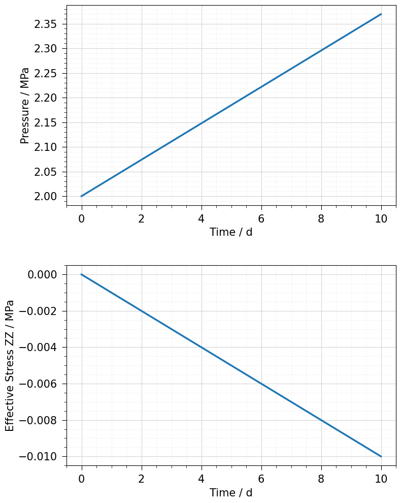
The obtained variations of pressure and effective stress at the end of the computation are shown in the two figures below:

fig, ax = plt.subplots(nrows=2, ncols=1, figsize=(8, 10))… (click to toggle)

fig, ax = plt.subplots(nrows=2, ncols=1, figsize=(8, 10))
ot.plot.line(ms_pts, "time", ot.variables.pressure, ax=ax[0], fontsize=15)
ot.plot.line(ms_pts, "time", ot.variables.stress["zz"], ax=ax[1], fontsize=15)
ax[0].set_xlabel("Time / d")
ax[0].set_ylabel("Pressure / MPa")
ax[1].set_xlabel("Time / d")
ax[1].set_ylabel("Effective Stress ZZ / MPa")

plt.tight_layout()
plt.subplots_adjust(hspace=0.3)
plt.show()

png

This article was written by Wenqing Wang & Noor Hasan. If you are missing something or you find an error please let us know.
Generated with Hugo 0.154.5 in CI job 743084 | Last revision: February 10, 2023