Example of a DGM-to-model-workflow
Workflow description
This documentation describes an exemplified workflow to create a groundwater flow model based on available data of a digital elevation model (here SRTM data ) and bathymetry data (here GPDN ). As tools, it uses a GIS (here QGIS ), the OGS DataExplorer and several OGS tools , as well as the meshing tool Gmsh and visualization tool ParaView . The first part of this documentation deals with the GIS work, the second with the OGS model setup.
GIS data preparation and extraction
This part will prepare the DGM and bathymetry data as input for the model setup. For all the QGIS editing steps, you may additionally define an output file (but this is no requirement); if this is not defined, QGIS will load the results into the active project.
Prepare elevation data
- It is likely that you will need to download more than one remote sensing image when the study area is large or overlapping the borders of one section. Download the required DGM data (here
.tiffiles) of the study area and load them into QGIS.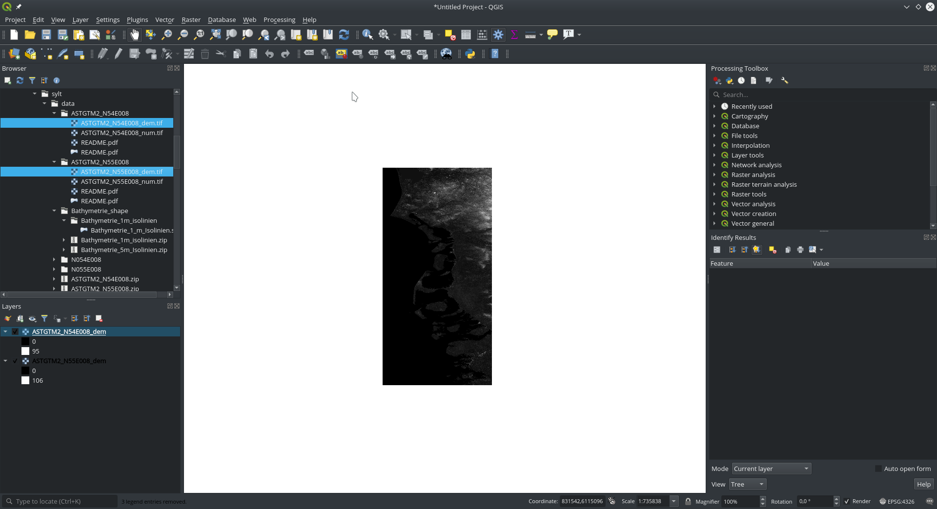
- Merge the images with
Raster->Miscellaneous->Merge...; select theInput Layers.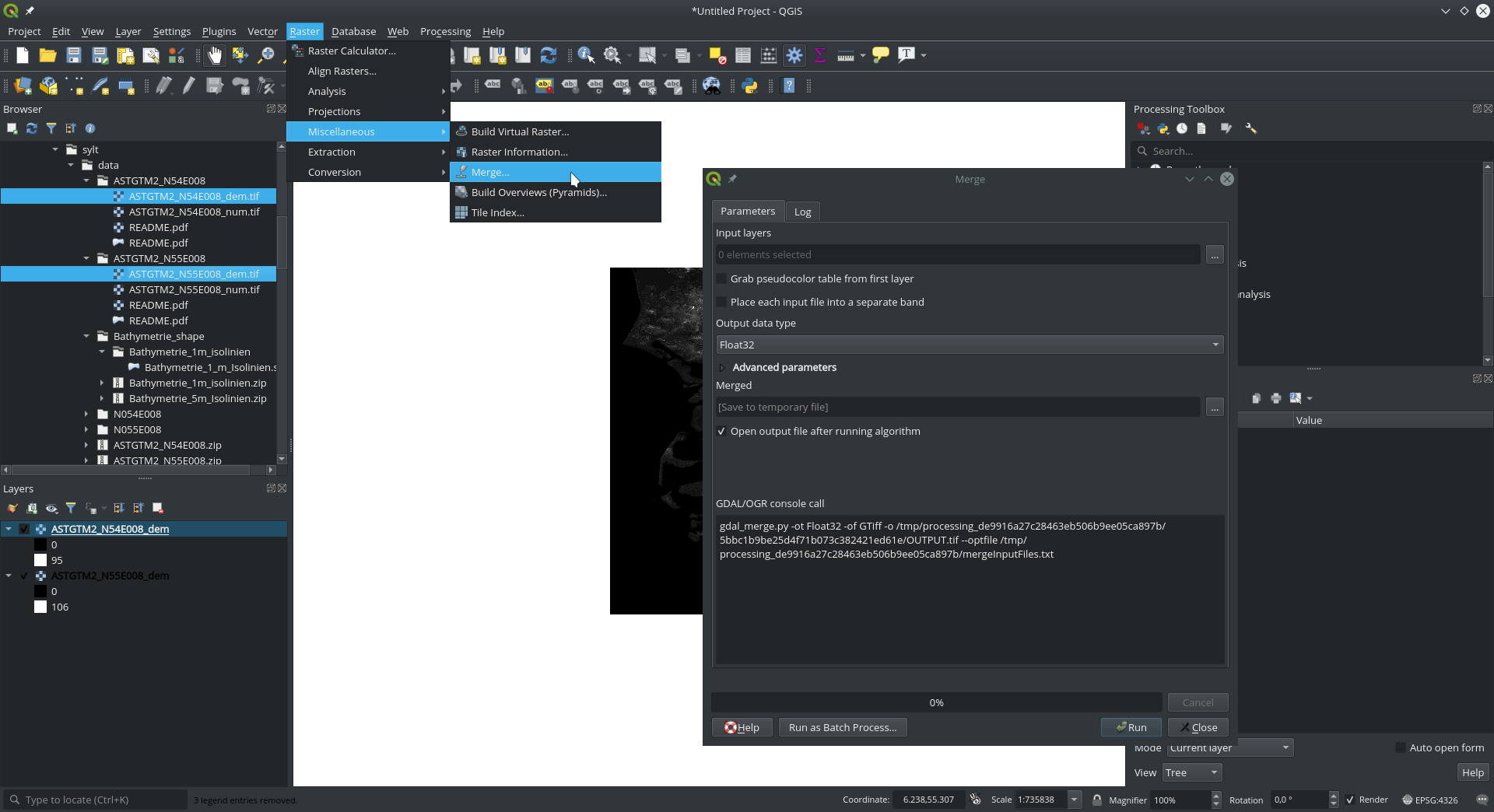
- Extract a subregion of the (merged) DGMs and define the study area through a shape file. One may also use a predefined shape file and continue with step 5. Choose
New Shapefile Layer...from the toolbar and enter aFile nameand a projection.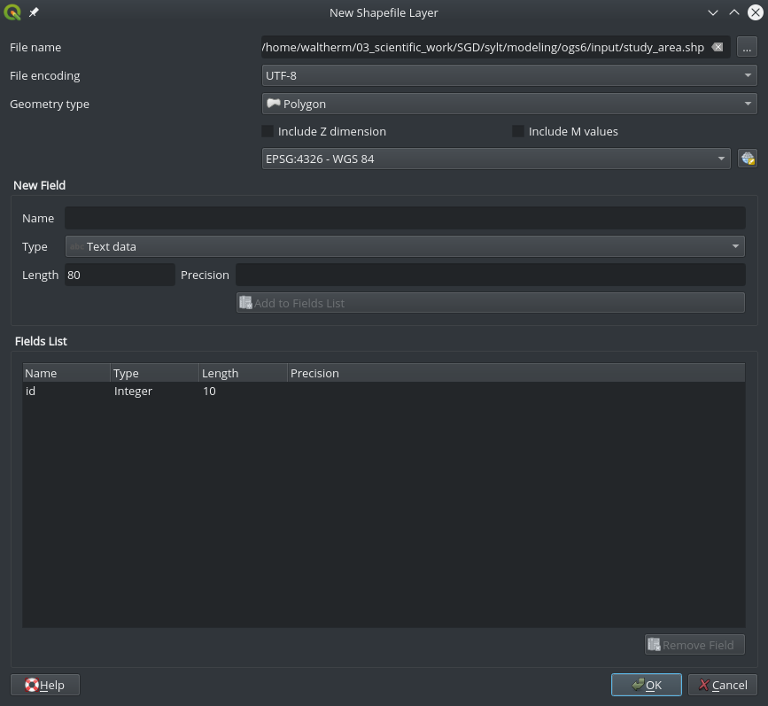
- Edit the shape (
Toggle Editingin toolbar), add points, and save the layer edits.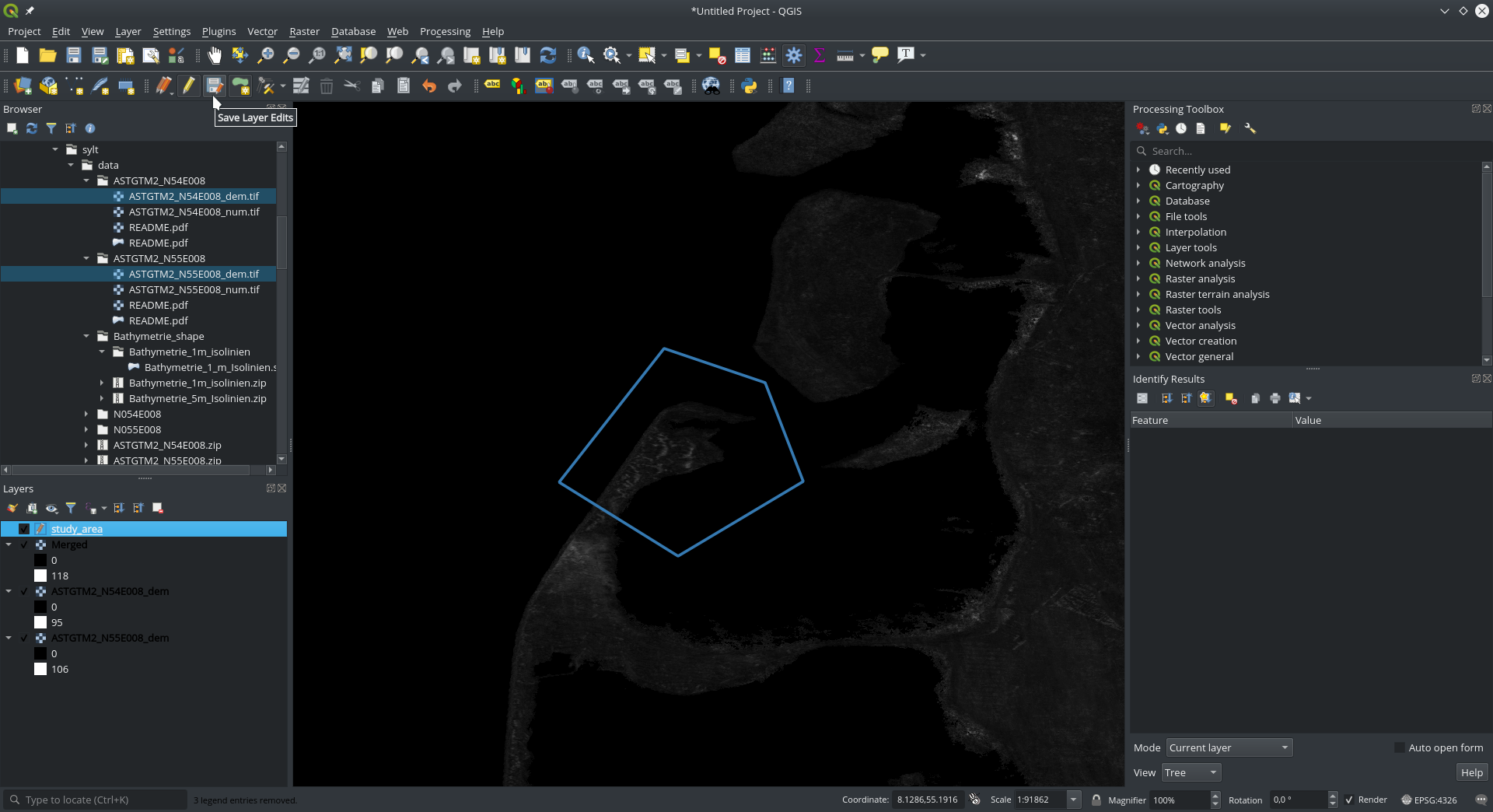
- Clip the DGM with the shape file with
Raster->Extraction->Clip Raster by Mask Layer...; defineInput LayerandMask layer, and assign theNodata value.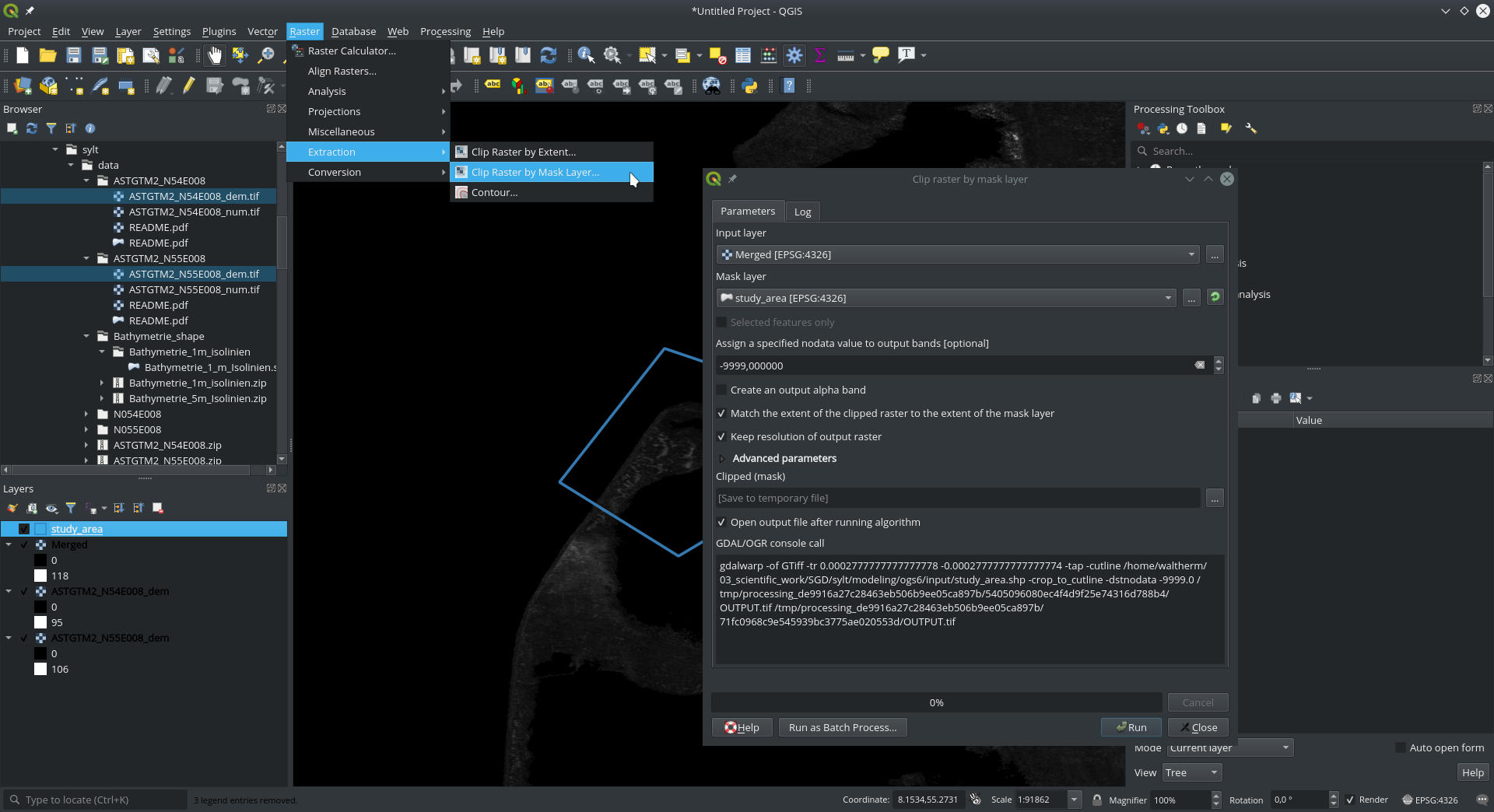
- If the raster does not have the correct projection, you will have to reproject it with the appropriate target system with
Raster->Projections->Warp (Reproject); select theInput Layerand theTarget CRS.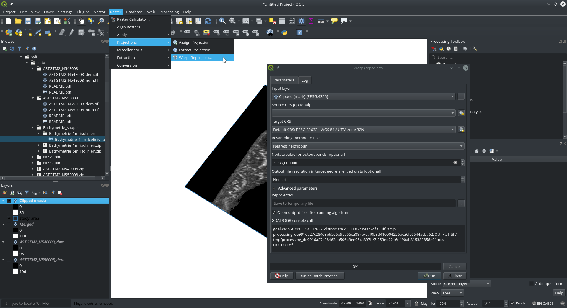
- This example also includes bathymetry data, which was available as vector data (isoline in a shape file). This file must be reprojected to the same coordinate system as the raster before with
Vector->Data Management Tools->Reproject Layer; selectInput Layerand theTarget CRS.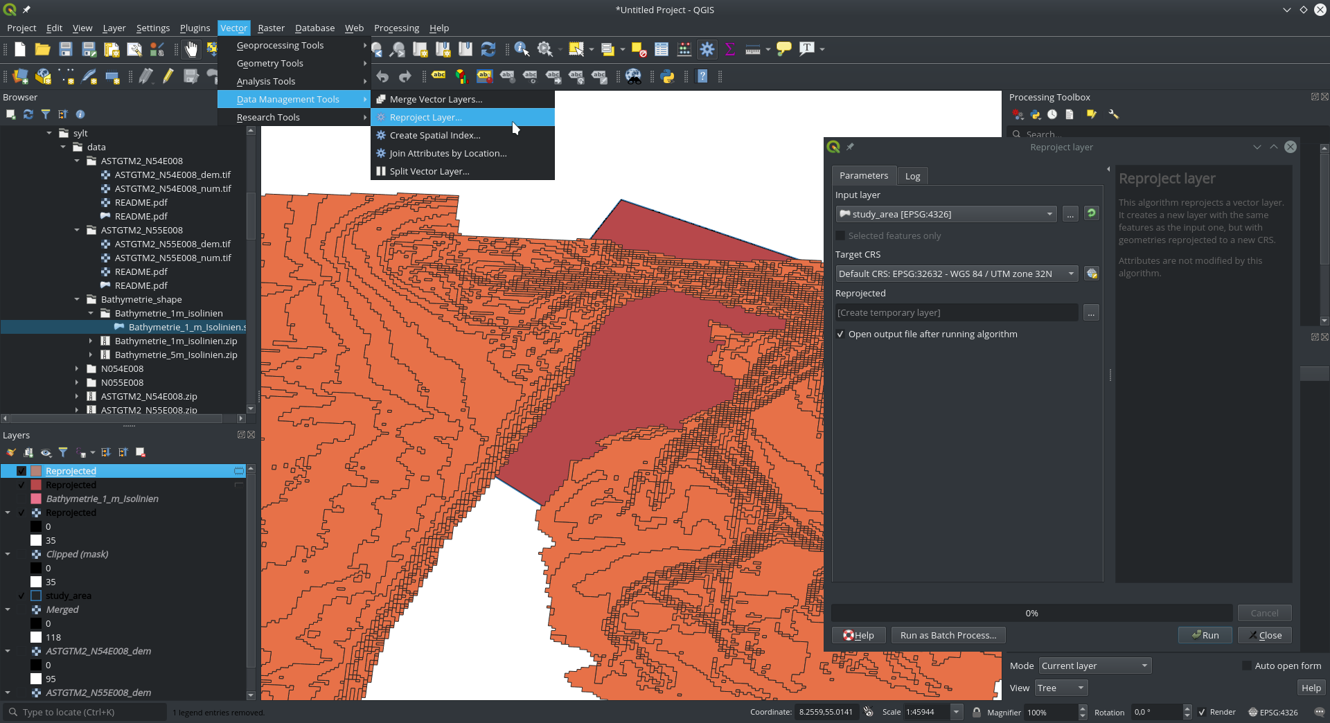
- Before merging DGM and bathymetry, the shape data needs to be converted to raster data with
Raster->Conversion->Rasterize (Vector to Raster); defineInput Layer, the z-value (burn-in value), the resolutions, and thenodata value.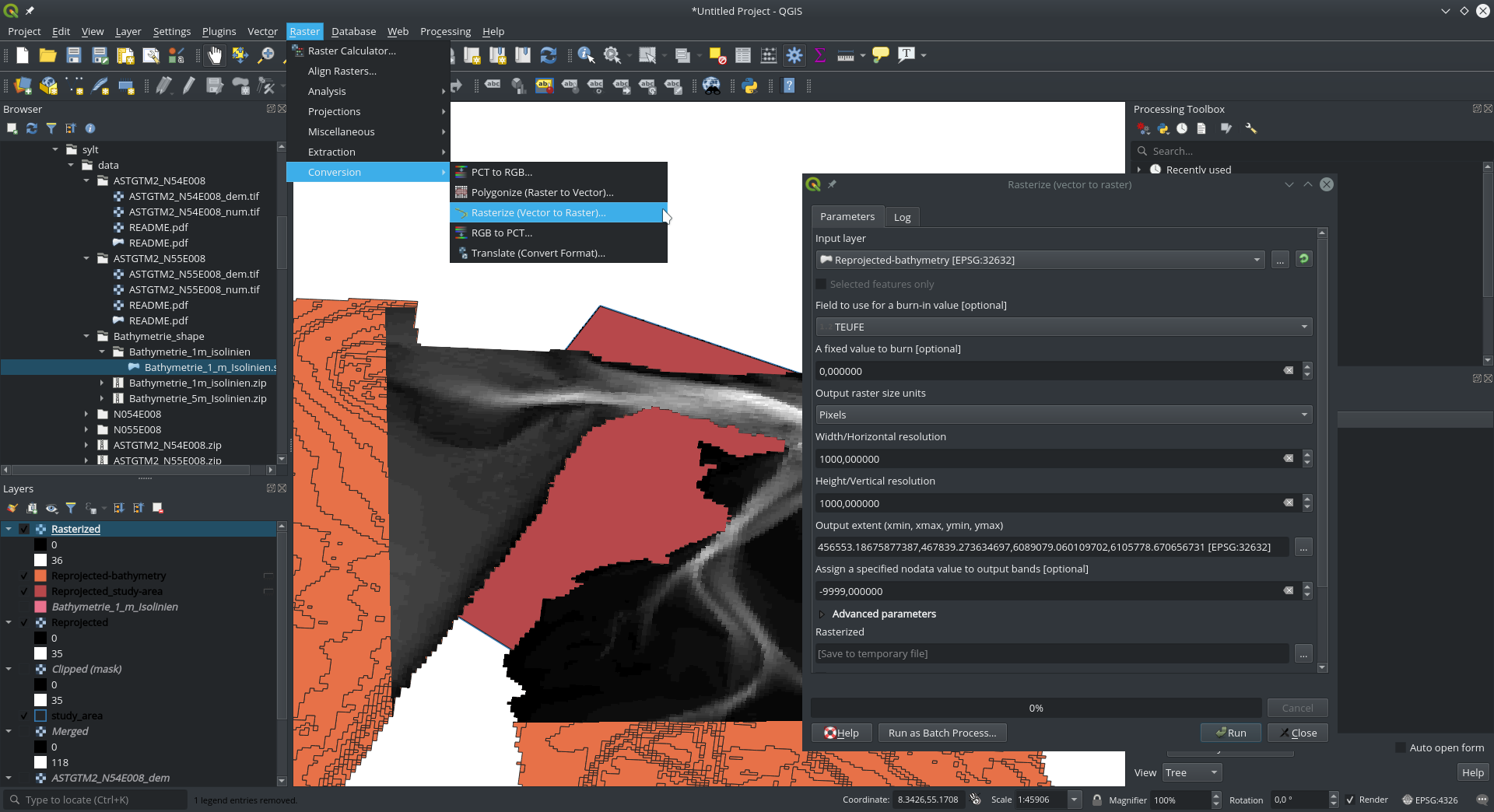
- As bathymetry was given as “depth”, this parameter needs to be converted to an “elevation”; use
Raster->Raster Calculatorand define theOutput layer, theOutput formatand theRaster Calculator Expression(shown formula only inverts the sign).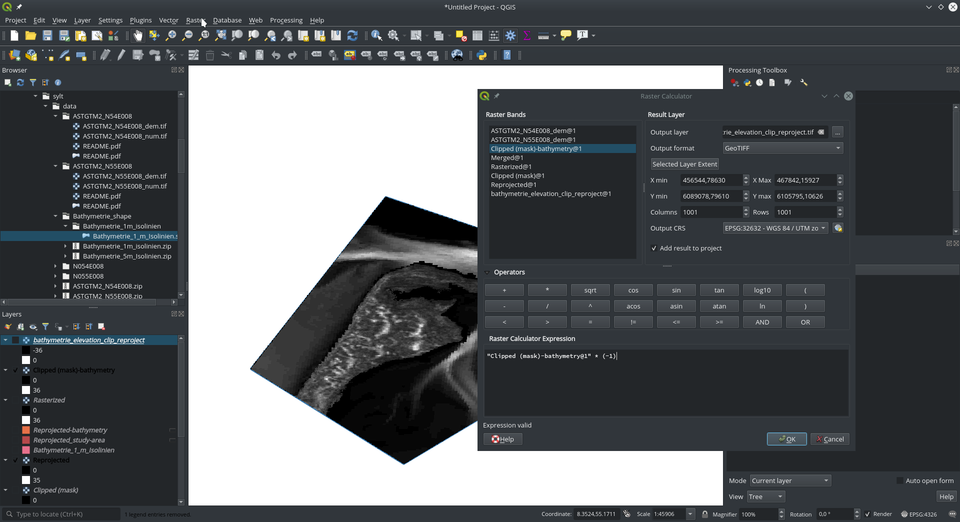
- Merge the DGM and bathymetry rasters (as done in step 2), and save the merged file as a
.ascfile withRaster->Conversion->Translate (Convert Format); define theInput Layerand theConvertedoutput file.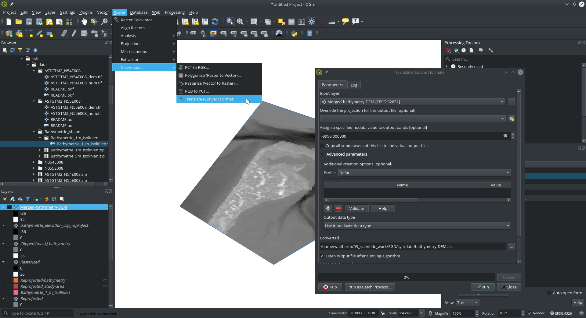
Prepare study area features
- To make the coastline part of the mesh, the merged DGM-bathymetry will be used to create a contour isoline at an elevation of
0.01 mwithExtraction->Contour...; select theInput Layer, set theInterval between contour linesto a high value and set theOffset from zero.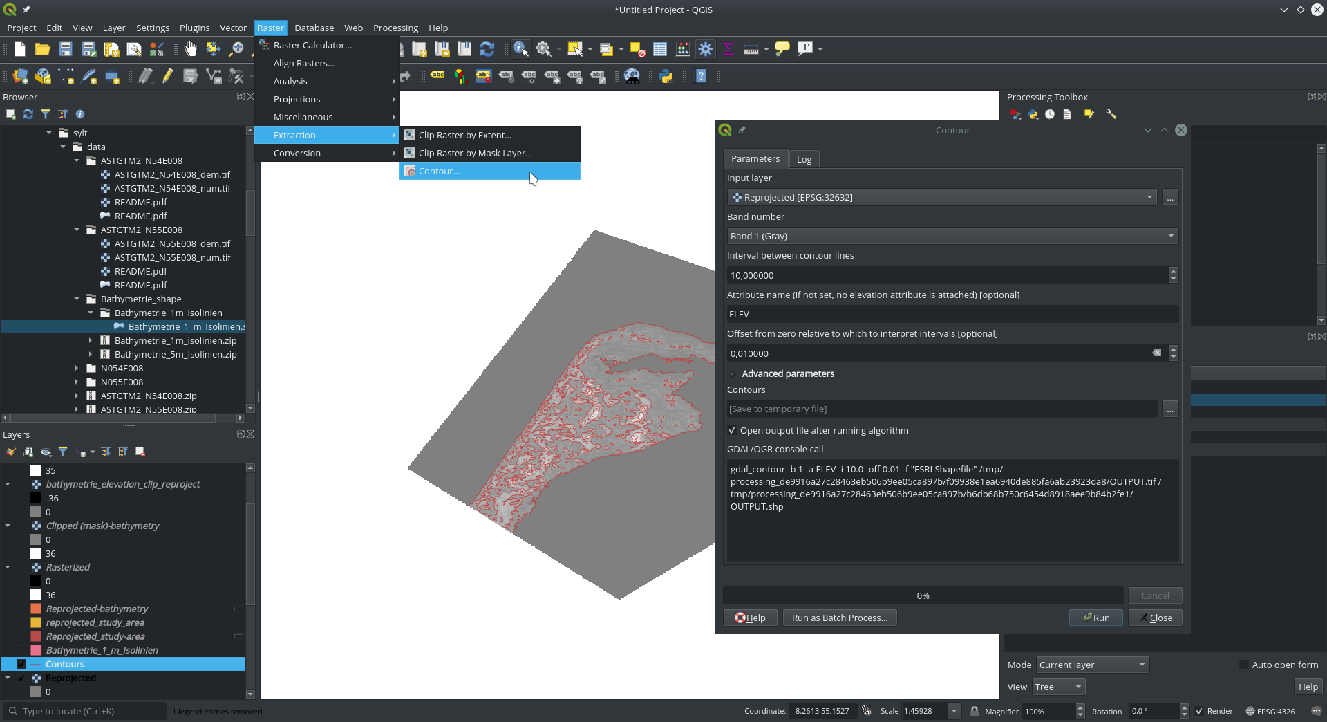
- If more than the
0.01 mcontour is present in the new shape file, remove the not required contours by right-clicking the new shape file andOpen Attribute Table; clickSelect features using an expressionand define the contours based on your liking that you want to exclude (here, anything with an elevation larger than 1 is removed).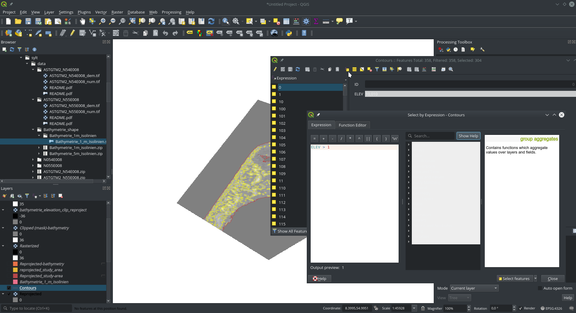
- Finish the selection (close attribute table) and remove the selected features by editing the shape (
Toggle Editing) and clickingDelete Selected; save the changes.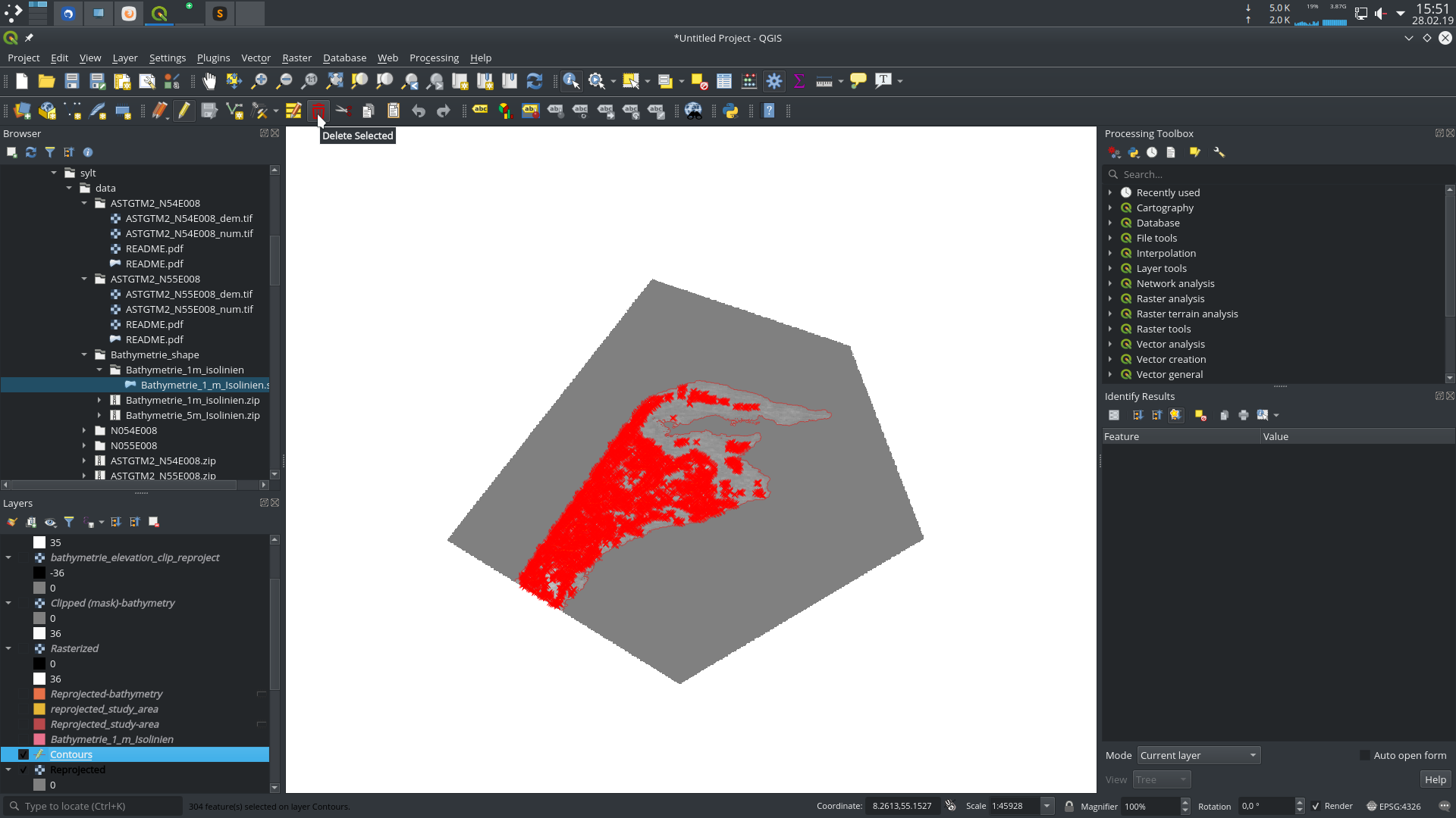
- The remaining features may have a high resolution (see red line in below figure); choose
Vector->Geometry Tools->Simplify..., and select anInput Layeras well as theSimplification methodwith an appropriateTolerance.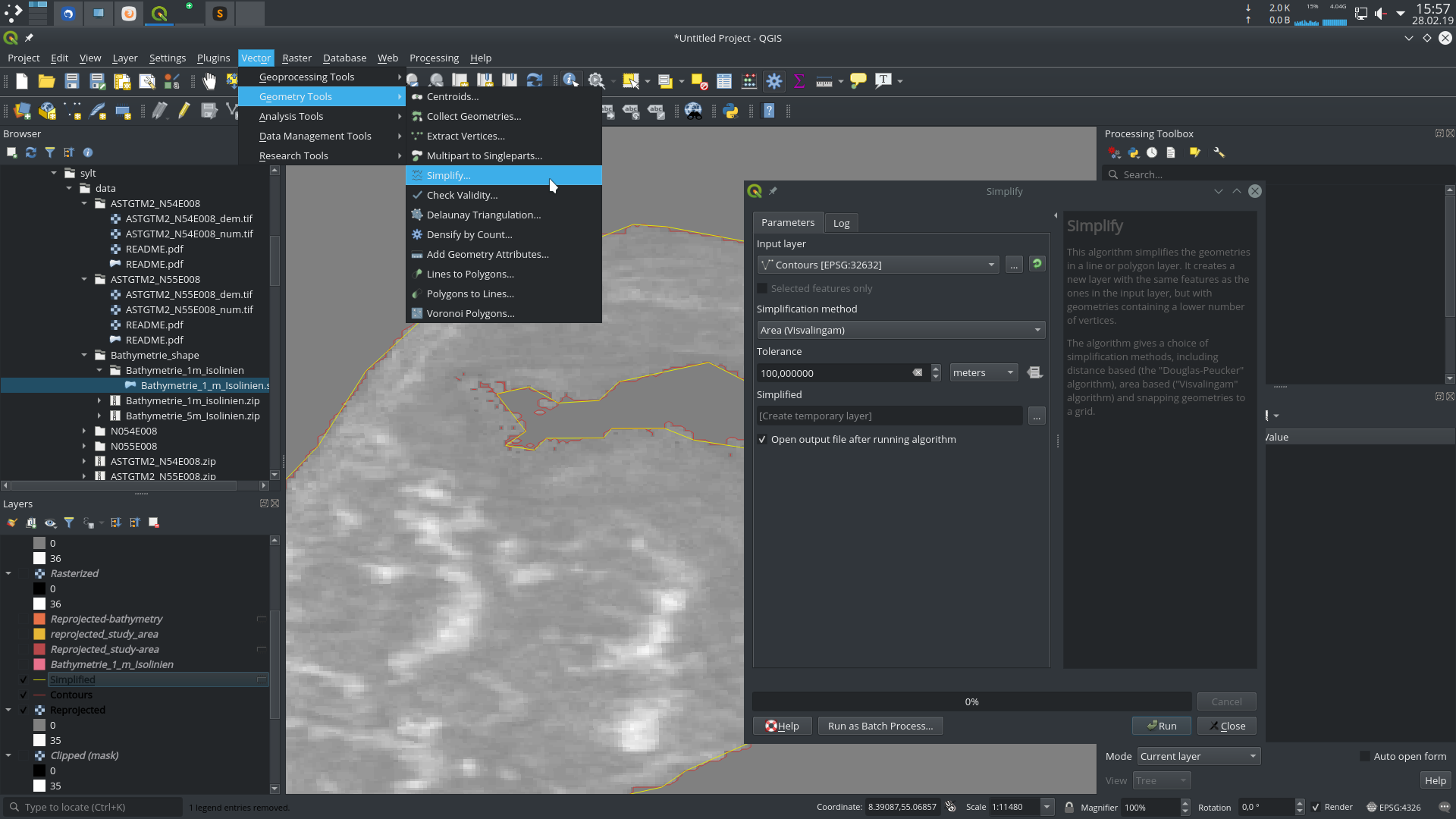
- Further, it might be useful to manually remove even more vertices from the polygon;
Toggle Editingof the simplified shape and select and remove vertices.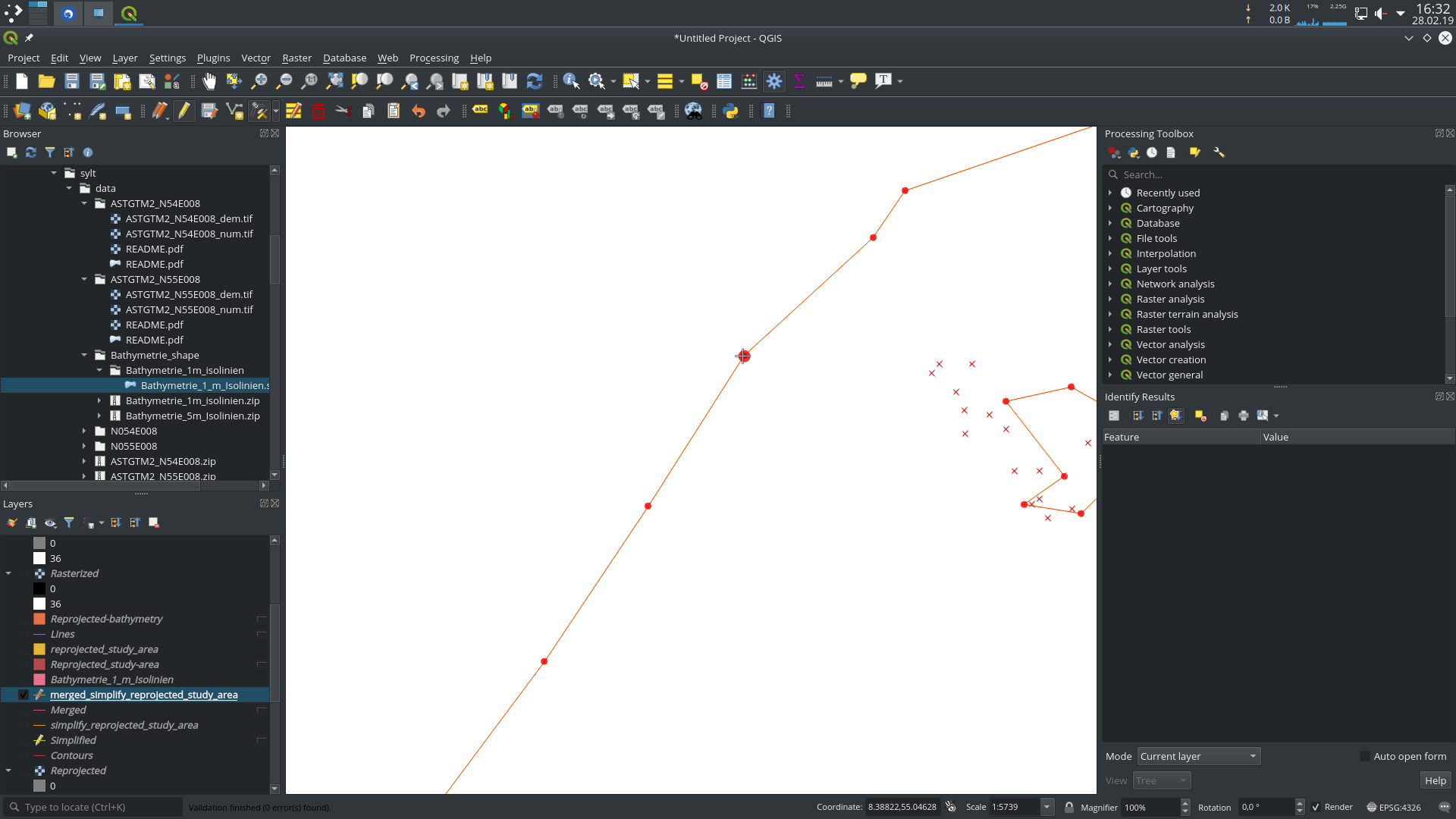
- The shape file used to clip the study area in step 5 will be used as the boundary of the model setup and be combined with the coastline. Firstly, convert the polygon of the study area to a polyline with
Vector->Geometry Tools->Polygons to Lines; select theInput Layer.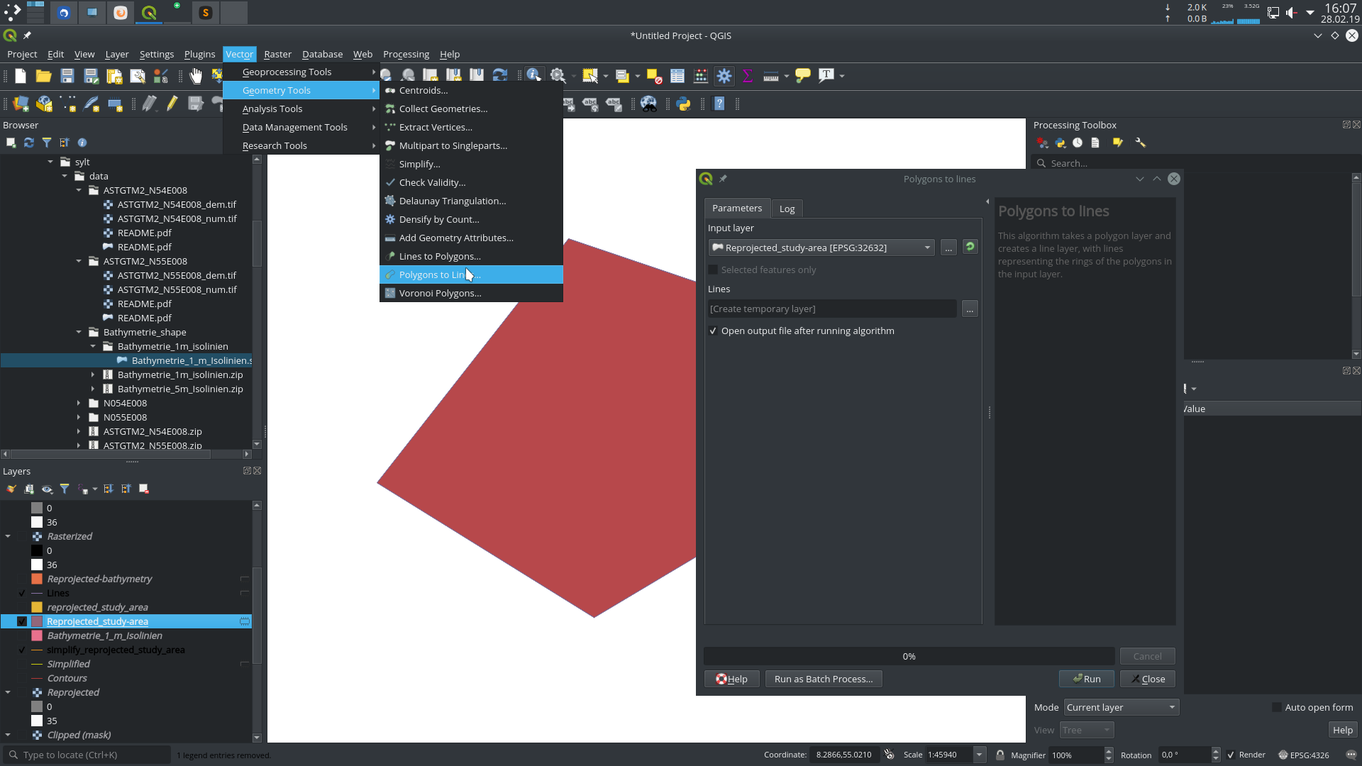
- Before merging the boundary and the coastline shapes, remove all fields from the boundary polyline through the
Attribute Table; select everything and clickDelete field.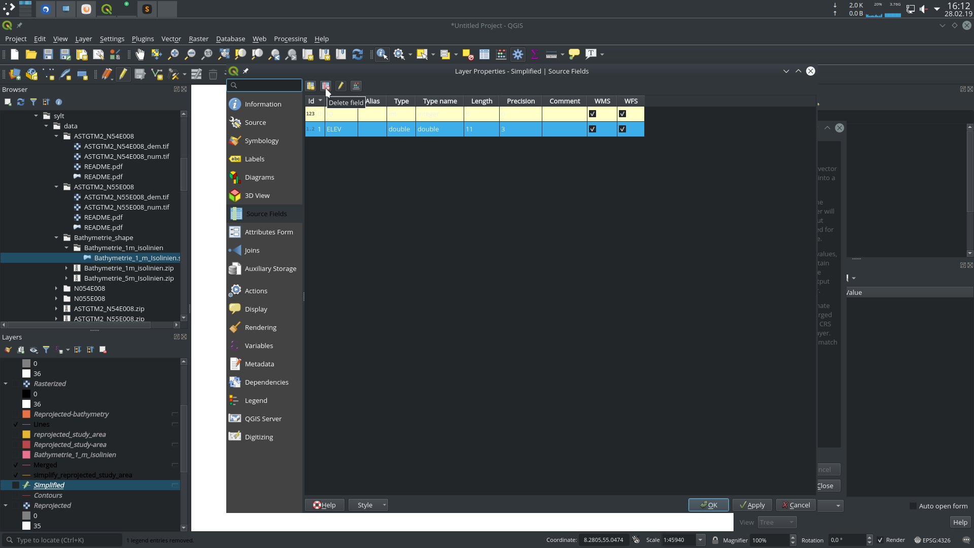
- Merge the boundary polyline and the coastline with
Vector->Data Management Tools->Merge Vector Layers; selectInput Layers.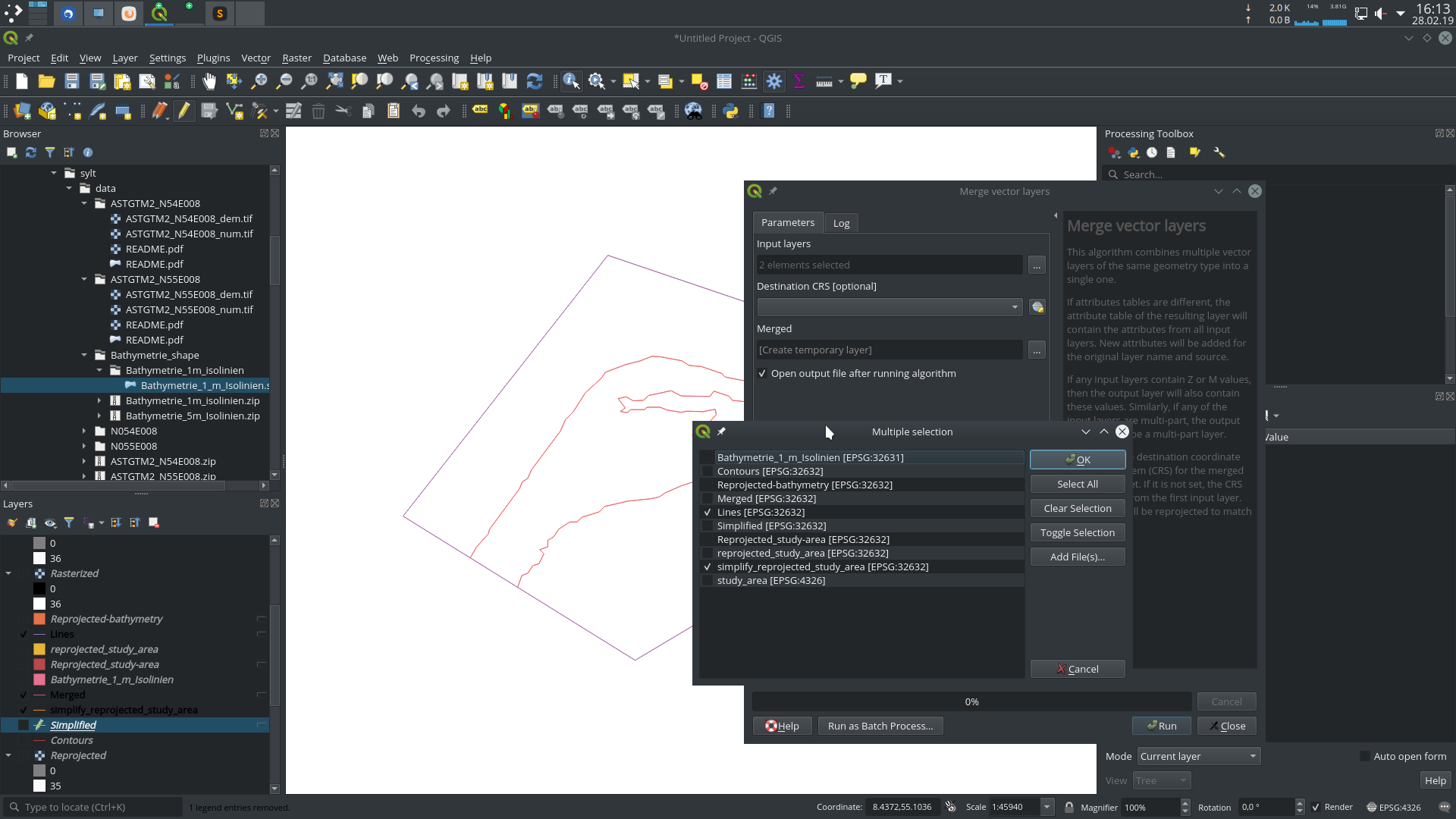
OGS model setup
The next steps will use the OGS DataExplorer, GMSH, and ParaView to prepare the model input files. A 2D mesh will be generated from the merged shape file containing the study area boundary and the coastline; the elevation data will be used to define the surface of the model and subsurface layer information will be used to define the aquifer structure.
3D Mesh creation
- Load the merged boundary-coastline shape into the DataExplorer (
File->Import->Shape Files). Creation of the 2D mesh can be done in two ways: a) Either use GMSH: Save the geometry as a.geofile for usage in GMSH by choosing the tabGeometryand clicking the save icon. Afterwards, use GMSH to generate a 2D mesh to your liking and import it withFile->Import Files->GMSH files....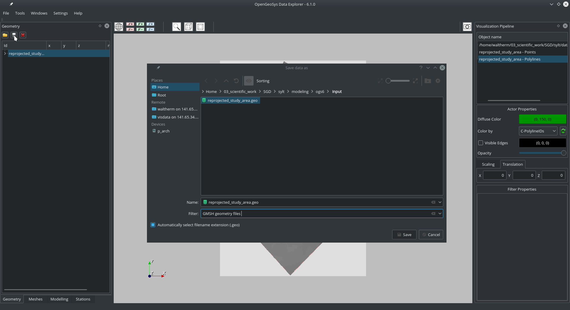 b) Or use the DataExplorer interface for GMSH: Use
 Tools->Create Mesh From Input Data....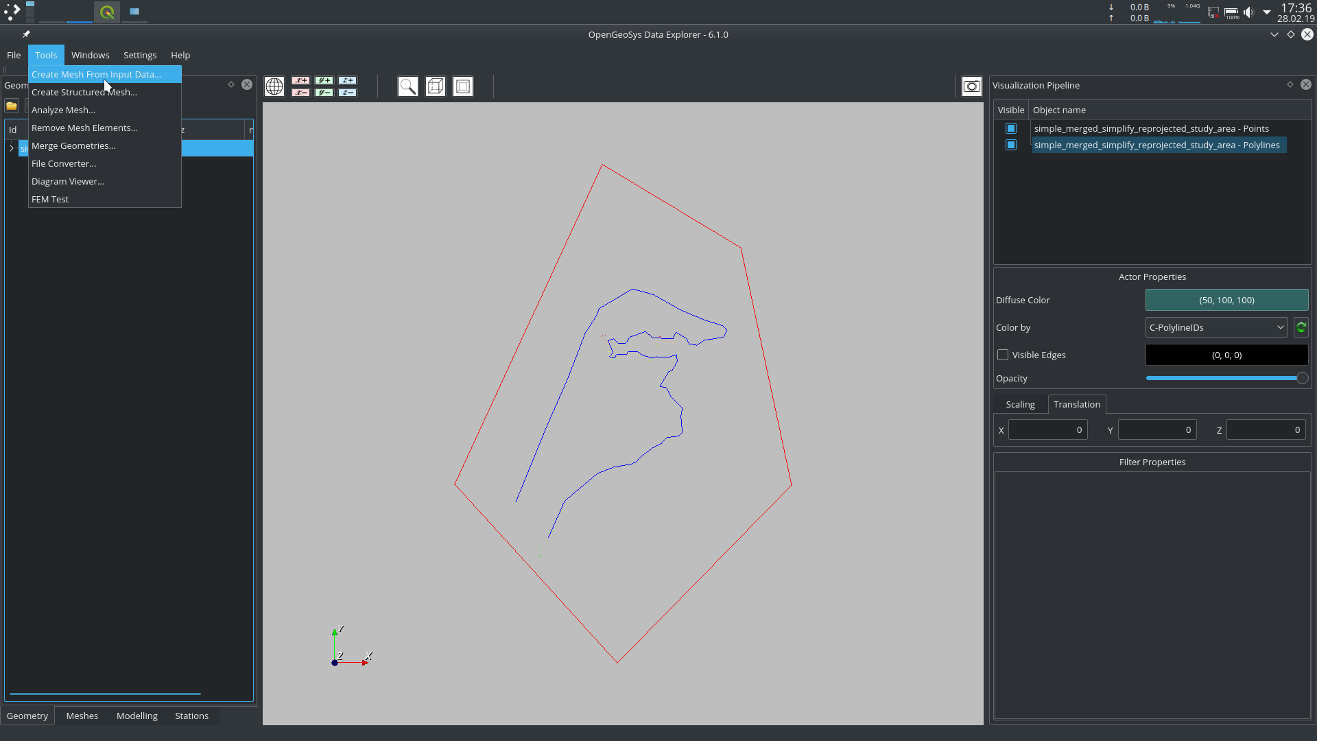 From the dialogue, select the geometry which should be used and let it show up on the right side (
Employed information).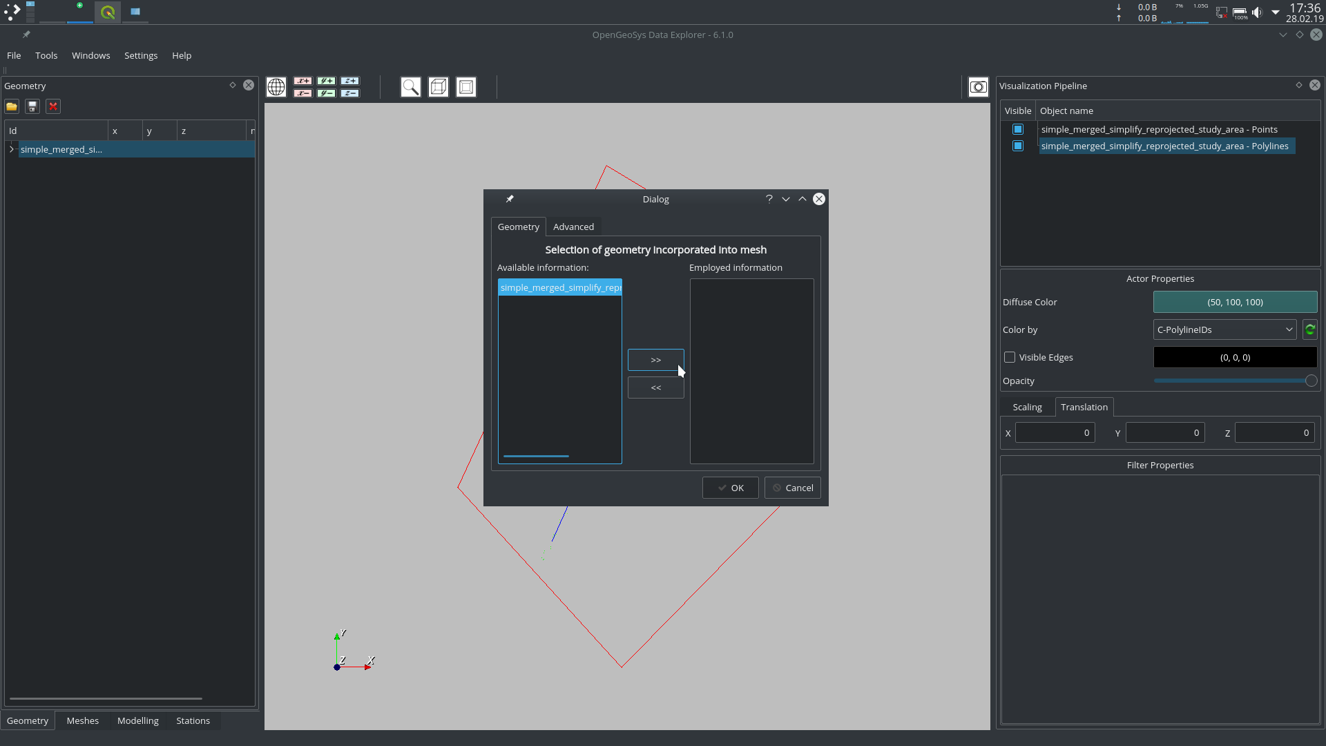 Select the
 Advancedtab, chooseAdaptive meshing, and remove the tick atDelete GMSH geo-file after generating mesh(in case you still want to manipulate the.geofile); clickOK.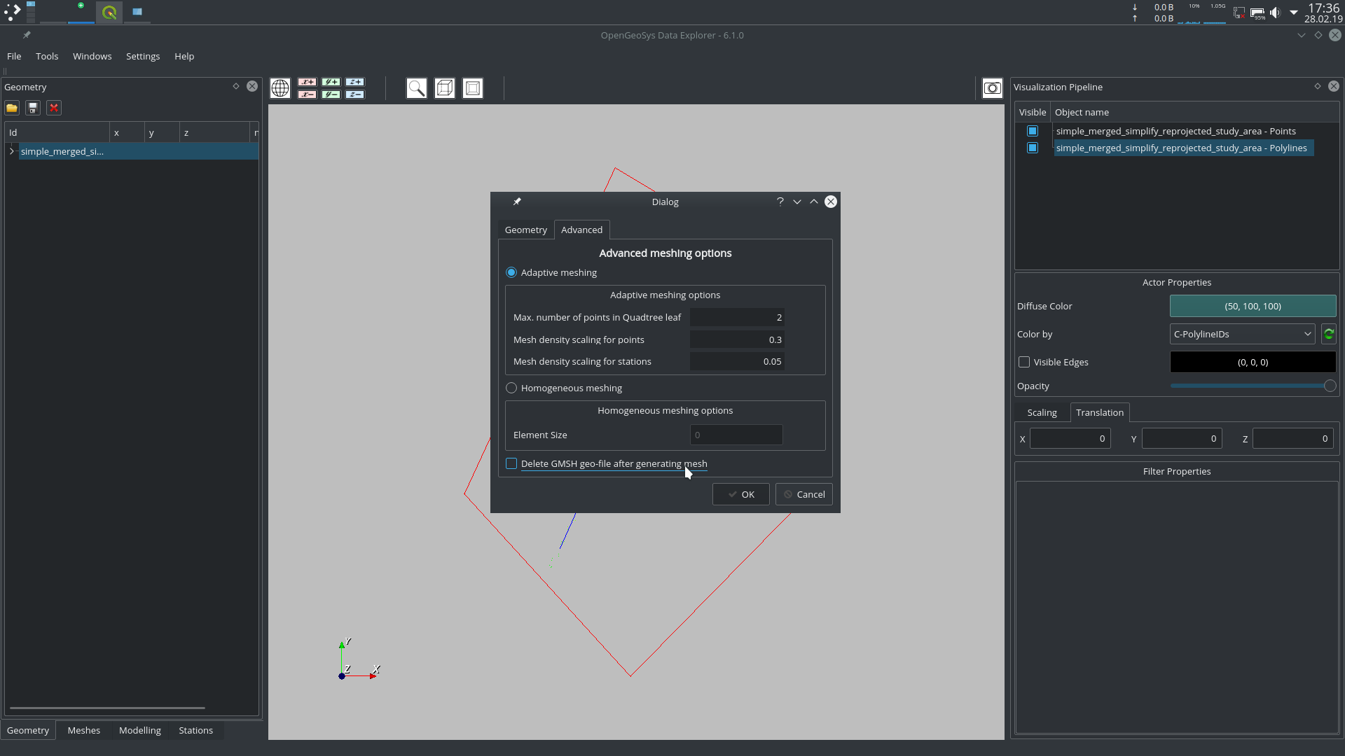
- To create a 3D mesh, the previously defined elevation data and subsurface layer data will be used to define multiple layers of the model. In the left-side tab
Meshes, right-click the newly created (or imported) mesh, and chooseEdit mesh...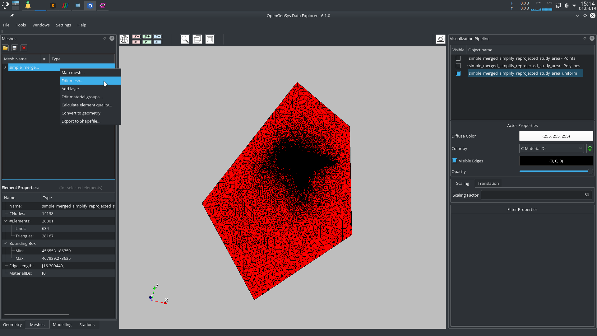
- In the new dialogue,
Specify the number of layers to add(here 10), clickAdd layers based on raster files, and load all.ascfiles that define the different layers into the interface. Also, define aMinimum thickness of layers(here 5 height units).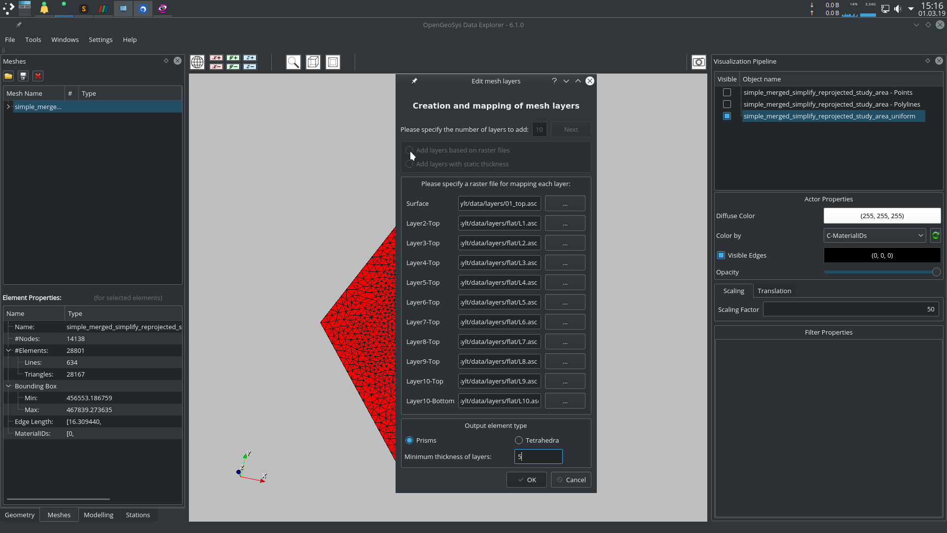
Boundary condition definition
For the creation of the boundary conditions, use the following workflow.
- Save the created 3D mesh as a
.vtufile by selecting the 3D mesh in theMeshestab and clicking the save icon. In the new dialogue, choose a output directory, filename, and theData mode.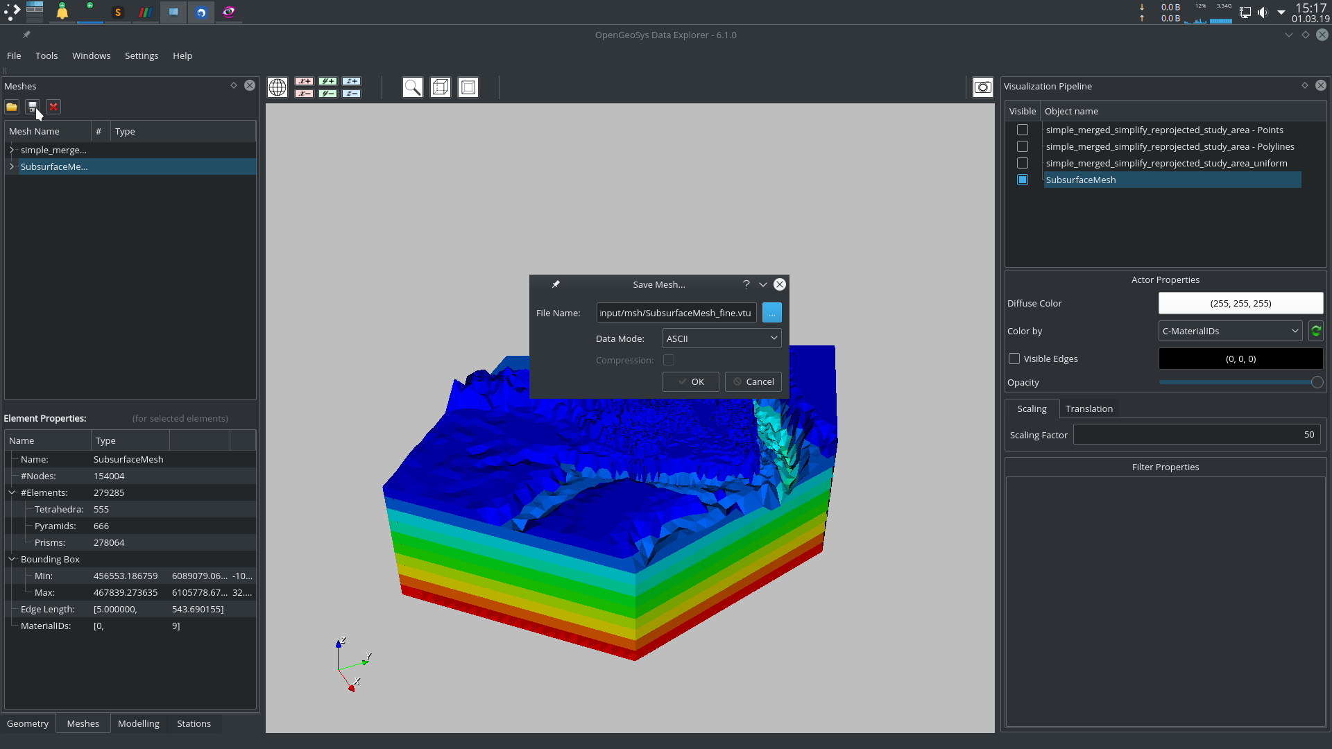
- To define water level and groundwater recharge, the top surface of the mesh will be used. Extract the surface with the tool
ExtractSurface. The following command is an example:ExtractSurface -i SubsurfaceMesh.vtu -o exSurf.vtu -x 0 -y 0 -z -1 -a 30 - ParaView will be used to define boundary and initial condition values.
For boundary conditions, a separation of the water level (Dirichlet) and recharge (Neumann) boundary condition is required. Load the extracted top surface into ParaView and apply the following filter pipeline:
a) Apply a
Calculatorwith the operationcoordsZto get a new parameter field with elevation data. b) Apply aThresholdand define the value range from the lowest to the water level (here -35 to 0.01 height units); this will be the input file for the Dirichlet boundary condition. c) Apply aCalculatorwith the operation-9810*coordsZ(i.e. fluid density multiplied by gravity by elevation) to get a pressure gradient. d) repeat b) and c) on theCalculatorfrom a) but with the value range water level to highest value (in theThreshold), and define the recharge value for the land area (in theCalculator). e) Save the “land” and “water” meshes as.vtufiles.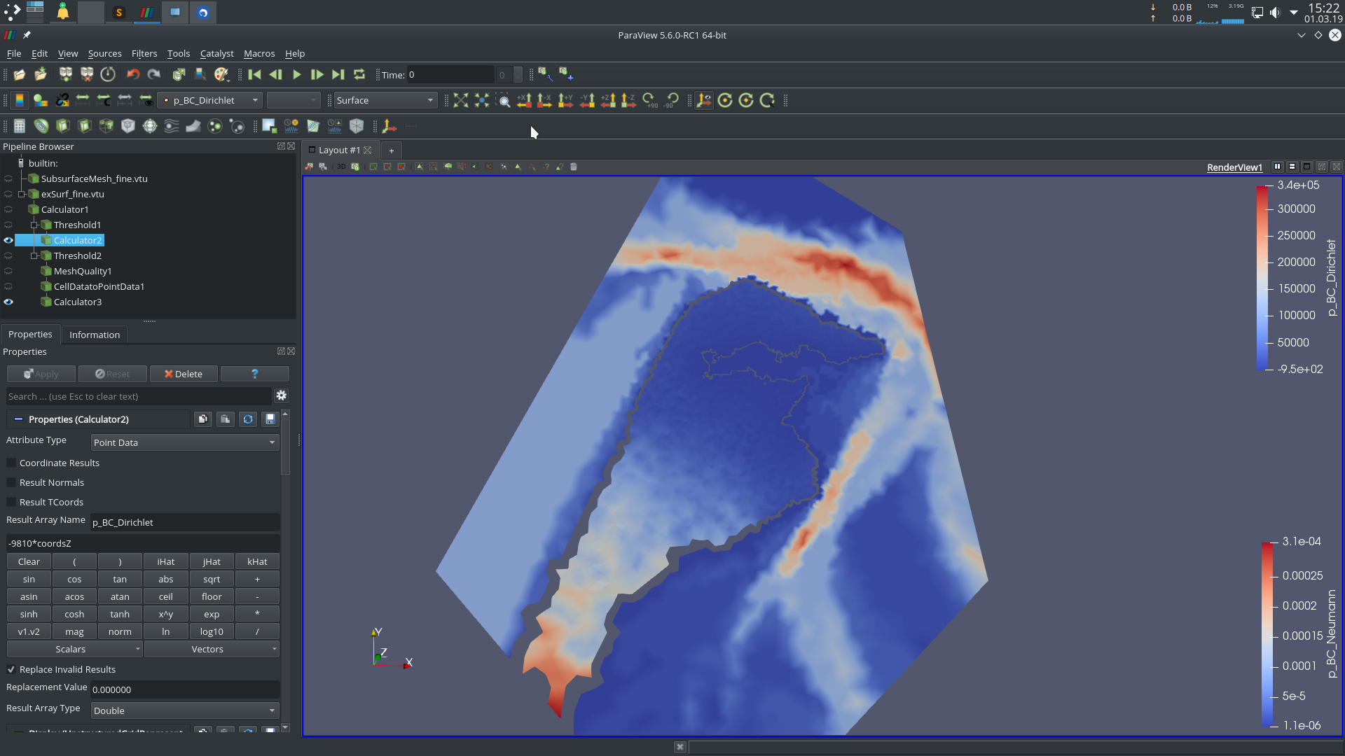
- Define the
.prjfile of your setup, including the 3D mesh and boundary condition meshes and run the simulation.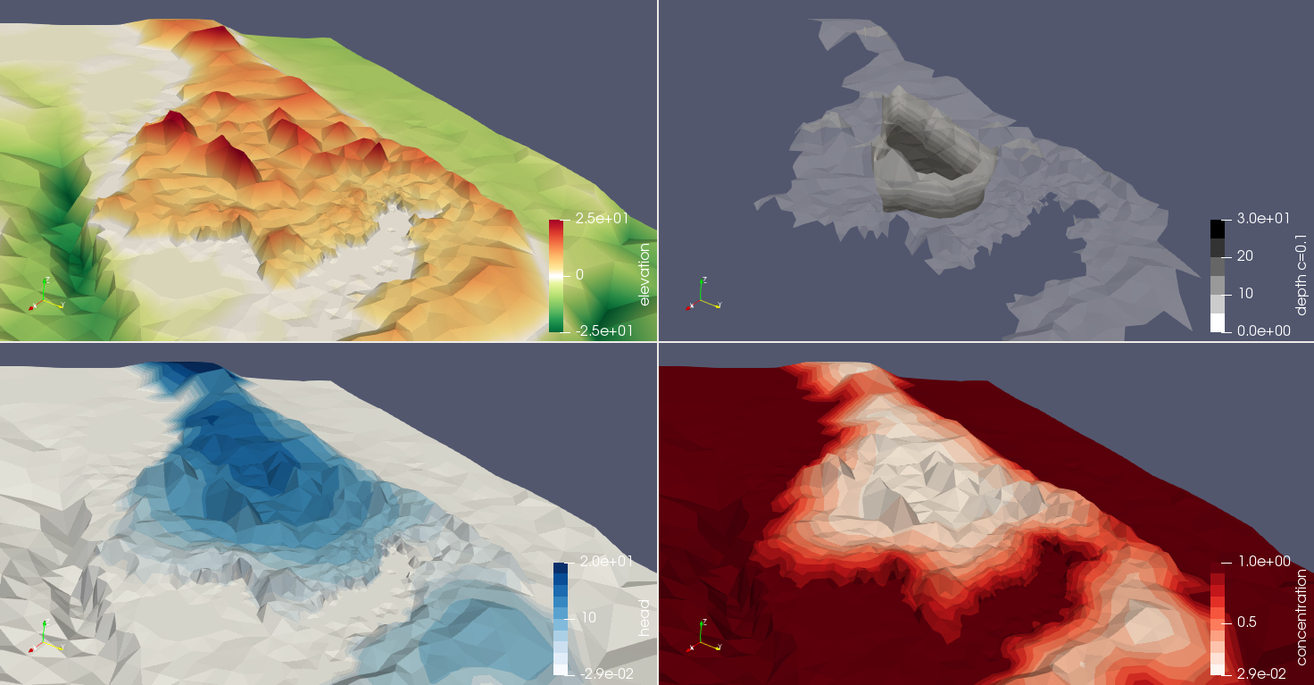
This article was written by Marc Walther. If you are missing something or you find an error please reach out
to us on our forum.
Generated with Hugo 0.164.0
in CI job 825193
|
Last revision: April 20, 2026
Commit: refactor(MeshLib): remove PropertyVector::push_back 870422dde
| Edit this page on