HEAT_TRANSPORT_BHE PipeNetwork Feature
Introduction
In a large borehole heat exchanger (BHE) array, all BHEs are connected with each other through a pipeline network. As the circulating fluid temperatures within each BHE are controlled by the network, the array itself has an intrinsic feature of balancing thermal extraction rates among different BHEs. This leads to the BHE thermal load shifting phenomena in the long-term operation. In OGS-6, this process can be simulated by using the PipeNetwork feature in the HEAT_TRANSPORT_BHE process.
This short tutorial aims to give the user a guide to the PipeNetwork feature. It includes the following main parts:
- The basic requirements for the PipeNetwork feature.
- The workflow of creating a pipeline network model using the software TESPy.
- The workflow of connecting the TESPy pipeline network model with the OGS model.
Requirements on the computer
In order to use the PipeNetwork feature, the computer running the HEAT_TRANSPORT_BHE process of OpenGeoSys is required to have a Python 3 environment with the TESPy program installed. For the Python 3 environmental installation, there are various tutorial available on the Internet. For the TESPy package, one can install it with the following command line in the Python3 environment:
pip3 install "tespy>=0.11,<0.12" iapwsThe iapws package provides the IAPWS-IF97 water properties used by the benchmark networks. See Fluid properties inside OGS
below for why the networks do not use TESPy’s default CoolProp back end.
Creating a pipeline network model with the software TESPy
Thermal Engineering Systems in Python (software paper: https://doi.org/10.21105/joss.02178
, software archive: https://doi.org/10.5281/zenodo.2555866
) is a software package developed by Francesco Witte. It is capable of simulating coupled thermal-hydraulic status of working fluids in thermal engineering applications. Such system typically involves a circulation network that is composed of pre-defined components including pipes, heat exchangers and different types of turbo machinery. Interested readers may refer to the online documentation (https://tespy.readthedocs.io/en/main/
) of TESPy for more detailed introduction of the software. The workflow in this part is built based on the benchmark example “A 3-BHE Array Coupled With Pipe Network” from the OpenGeoSys Documentation (https://www.opengeosys.org/docs/benchmarks/heat-transport-bhe/3d_3bhes_array/
). One can refer to this benchmark and download its latest benchmark files from GitHub (https://www.opengeosys.org/docs/userguide/basics/introduction/
) for creating the pipeline network TESPy model. This tutorial follows the TESPy 0.11 API; it is tested with TESPy 0.11.x. The complete, runnable version of the script shown below is Tests/Data/Parabolic/T/3D_3BHEs_array/pre/3bhes_closedloop.py.
The coupled model that is going to be built is demonstrated in Figure 1. It consists of a pipeline network connected with 3 BHEs, a water pump, a virtual heat pump as the consumer, a splitter to split up the feeding fluid flow and a merge to returned flow. These devices are all defined as components in TESPy. A full list of available components can be found in the TESPy components module. In the pipeline network, these components are connected with each other through connections parts, which are illustrated by the black lines in the figure. With these two main parts, a completely TESPy pipeline network model can be set up.

Pipeline network model in TESPy
< Network >
Firstly a network needs to be created. It is the main container for the model. Several parameters will be set here, for example the unit systems for the networks variables. Since TESPy 0.9 the fluids are no longer declared on the network; they are set per connection instead (see below).
from tespy.networks import Network
from tespy.connections import Connection, Ref
from tespy.components import Source, Sink, Pump, Splitter, Merge, SimpleHeatExchanger, CycleCloser
from tespy.tools.characteristics import CharLine
from tespy.tools.fluid_properties.wrappers import IAPWSWrapper
import numpy as np

# %% network
btes = Network()
btes.units.set_defaults(
    temperature='K', pressure='bar', pressure_difference='bar', enthalpy='kJ / kg'
)Units are configured through Network.units.set_defaults(). Passing them to the Network constructor, as TESPy 0.3 required, raises a TypeError from TESPy 0.10 onwards.
<Components>
In the next step different components in the network needed to be configured. In TESPy model the fluid usually emerges from a Source and drains in a Sink term. However, a virtual loop system is created by using the component CycleCloser. This component ensures, that enthalpy and pressure at the Source and the Sink are identical. In our model, TESPy components of type CycleCloser, Pump, Splitter, Merge and SimpleHeatExchanger are created with locally defined names surrounded by quotes. To simplify the model the heat pump is specified as a pure heat exchanger to consume the heat.
# %% components
fc = CycleCloser('cycle closer')
pu = Pump('pump')
sp = Splitter('splitter', num_out=3)

# bhe:
bhe1 = SimpleHeatExchanger('BHE1')
bhe2 = SimpleHeatExchanger('BHE2')
bhe3 = SimpleHeatExchanger('BHE3')

mg = Merge('merge', num_in=3)
cons = SimpleHeatExchanger('consumer')When all components are set up, it is needed to specify parameters for them. One can find the full list of parameters for a specific component in the respective TESPy class documentation. In this model, a pump curve for the water pump, physical properties (length, diameter, roughness) for the BHE pipes, the imposed thermal load on the virtual heat pump are specified as follows.
## components parameterisation
# pump
# flow_char
# provide volumetric flow in m^3 / s
x = np.array([
    0.00, 0.00001952885971862, 0.00390577194372, 0.005858657915586,
    0.007811543887448, 0.00976442985931, 0.011717315831173, 0.013670201803035,
    0.015623087774897, 0.017575973746759, 0.019528859718621, 0.021481745690483,
    0.023434631662345, 0.025387517634207, 0.027340403606069, 0.029293289577931,
    0.031246175549793, 0.033199061521655, 0.035151947493517, 0.037104833465379,
    0.039057719437241, 0.041010605409104, 0.042963491380966, 0.044916377352828,
    0.04686926332469, 0.048822149296552, 0.050775035268414, 0.052727921240276,
    0.054680807212138, 0.056633693184
])

# provide head in Pa
y = np.array([
    0.47782539, 0.47725723, 0.47555274, 0.47271192, 0.46873478, 0.46362130,
    0.45737151, 0.44998538, 0.44146293, 0.43180416, 0.4220905, 0.40907762,
    0.39600986, 0.38180578, 0.36646537, 0.34998863, 0.33237557, 0.31362618,
    0.29374046, 0.27271841, 0.25056004, 0.22726535, 0.20283432, 0.17726697,
    0.15056329, 0.12272329, 0.09374696, 0.06363430, 0.03238531, 0.00000000
]) * 1e5
char = CharLine(x=x, y=y)
pu.set_attr(flow_char={'char_func': char, 'is_set': True})
pu.set_attr(eta_s=0.90)

# bhes
bhe1.set_attr(D=0.013665, L=100, ks=0.00001)
bhe2.set_attr(D=0.013665, L=100, ks=0.00001)
bhe3.set_attr(D=0.013665, L=100, ks=0.00001)

# consumer
cons.set_attr(pr=1)
# consumer heat demand
cons.set_attr(Q=-3000) # WConnections
Connections are used to link two components. It starts from the outlet of the component 1 to the inlet of component 2. In order to connect all components with each other a system workflow sequence needs to be determined. In this case the fluid flowing from the inlet source term will be firstly lifted by the pump. Then the inflow will be divided into 3 branches by the splitter and then flow into each BHEs. After that the outflow from the BHEs will be mixed together at the merging point and then feed into the heat pump for heat extraction. The total sequence ends up when the flow reaches the outlet sink term. In the last step, all connections have to be added into the network container to form a complete network.
Each connection is given an explicit label. The labels are what identifies a connection when the network is written to and read back from JSON, so they should be set even though TESPy would generate one automatically.
# connections
fc_pu = Connection(fc, 'out1', pu, 'in1', label='fc_pu')
pu_sp = Connection(pu, 'out1', sp, 'in1', label='pu_sp')

sp_bhe1 = Connection(sp, 'out1', bhe1, 'in1', label='sp_bhe1')
sp_bhe2 = Connection(sp, 'out2', bhe2, 'in1', label='sp_bhe2')
sp_bhe3 = Connection(sp, 'out3', bhe3, 'in1', label='sp_bhe3')

bhe1_mg = Connection(bhe1, 'out1', mg, 'in1', label='bhe1_mg')
bhe2_mg = Connection(bhe2, 'out1', mg, 'in2', label='bhe2_mg')
bhe3_mg = Connection(bhe3, 'out1', mg, 'in3', label='bhe3_mg')

mg_cons = Connection(mg, 'out1', cons, 'in1', label='mg_cons')
cons_fc = Connection(cons, 'out1', fc, 'in1', label='cons_fc')

btes.add_conns(fc_pu, pu_sp, sp_bhe1, sp_bhe2, sp_bhe3, bhe1_mg, bhe2_mg,
bhe3_mg, mg_cons, cons_fc)Here the fluid properties within the connection is set to be identical. It means when two components are connected with each other, the fluid properties for instance the mass flow rate, the pressure, the temperature at the outlet of component 1 will be equal to the values at the inlet of component 2. In order to complete the calculation, several boundary conditions are required to be imposed on the connections. First, the inflow pressure is fixed. A temporary outflow temperature on each BHEs is specified to make sure the network is computable. In this case the consumed heat on the virtual heat pump is assumed to be totally supplied by the 3 BHEs. The cycle closer ensures, that pressure and enthalpy at the consumer’s outlet are identical to those at the pump’s inlet.
## connection parametrization
# system inlet
# The IAPWS-IF97 engine is used instead of TESPy's CoolProp default, because
# CoolProp crashes inside OGS's embedded Python. It is propagated from this
# connection to all others of the network.
fc_pu.set_attr(p=2, fluid={'water': 1}, fluid_engines={'water': IAPWSWrapper})

# for BHEs:
# Tout:
bhe1_mg.set_attr(T=303.15)
bhe2_mg.set_attr(T=303.15)
bhe3_mg.set_attr(T=303.15)Solve
After the network, components and connections are completely set up, the system can be solved to get its steady states results. One can use the print_results to find the details parameters during the calculation.
# %% solve
btes.solve('design')
#btes.print_results()Save the network
At last, the built BHE pipe network model needs to be exported into the project working folder. Since TESPy 0.9 a network is written as a single JSON file with export() (the older save(), which produced a directory of CSV files, is gone).
# %% save to json:
btes.export('tespy_nw_closedloop.json')Fluid properties inside OGS
By default TESPy evaluates fluid properties with CoolProp. Loading CoolProp inside the Python interpreter embedded in OGS crashes, so the benchmark networks are configured for TESPy’s IAPWSWrapper instead, which uses the IAPWS-IF97 formulation from the iapws package.
Two small workarounds are needed on top of that, and they are collected in bhe_tespy_compat.py, which sits next to the boundary condition script in each benchmark directory:
- a stub
CoolPropmodule, installed before TESPy is imported, so that TESPy’s unconditional top-levelimport CoolPropdoes not load the real library; - a viscosity fallback for
IAPWSWrapper, becauseiapwsreturnsNonefor the dynamic viscosity of two-phase states, which the solver can transiently visit.
These are needed by the boundary condition scripts, which run inside OGS. The network generation scripts under pre/ run as ordinary Python and do not need them; they only have to select the IAPWSWrapper engine as shown above, so that the exported network uses it at run time.
A boundary condition script therefore has to install the workarounds before importing anything from tespy:
import bhe_tespy_compat

bhe_tespy_compat.install_workarounds()

from tespy.networks import NetworkConnecting the TESPy model with the OGS model
The work flow of the PipeNetwork feature is illustrated in Figure 2. To explicitly simulate both the BHE and the pipe network, OGS is coupled with the TESPy through a Python interface. Within every time step and each iteration, the outflow temperature Tout from each BHE is computed by OGS and transferred to TESPy via the interface. Then TESPy will use these Tout temperature and the current hydraulic state as the boundary condition imposed on the pipeline network to calculate the current inflow temperature Tin of each BHE and the currently flow rate, which satisfies the overall thermal load of the building. After the calculation, all data will be transferred back to OGS and update the inlet temperature and flow rate of each BHE for the next iteration. The convergence is set to be satisfied when the difference from the last two iteration results is smaller than a preset tolerance value. Additionally, OGS will transfer the currently time step ’t’ to TESPy within each iteration, which makes TESPy able to adjust its time dependent network boundary conditions according to the user’s configuration.
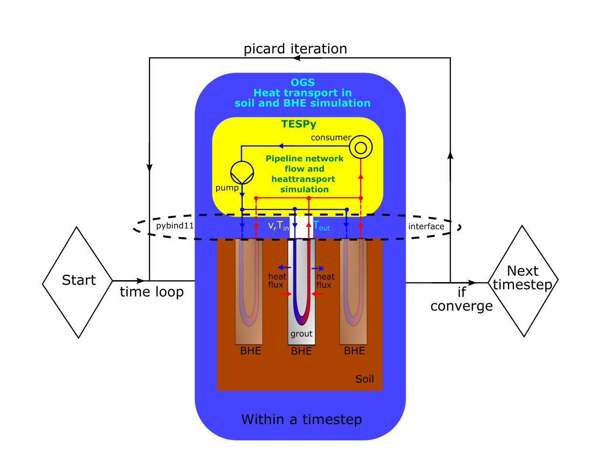
Work flow of the model with BHEs coupled with a pipe network
BHE data container
In order to use the PipeNetwork feature, the pre-built and saved TESPy network model in the above section is required. A CSV file bhe_network.csv which contains all the OGS-TESPy transferred BHE information needs to be created. The PipeNetwork feature will access this CSV file to initialize the exchange data container between OGS and TESPy during the simulation. All BHEs have to be included in this CSV file. Please take notice that all BHE names located in the data_index column have to be identical with the BHE names defined in the corresponding TESPy network model.
data_index;BHE_id;Tin_val;Tout_val;Tout_node_id;flowrate
BHE1;1;283.15;283.15;0;0
BHE2;2;283.15;283.15;0;0
BHE3;3;283.15;283.15;0;0PipeNetwork feature interface
The python script referenced from the project file is the data exchange interface for running the PipeNetwork feature.
It contains the main procedure of data exchange during the simulation.
The closed loop network built above is driven by bcs_tespy_closedloop.py; the one-way network built with a Source and a Sink is driven by bcs_tespy.py.
Both scripts are structured identically and differ only in the network file they load.
In the script a network status controller function network_status, a system dynamic thermal load function consumer_demand and a system dynamic inlet flow rate function dyn_frate are optionally required to be pre-defined by the user.
The function network_status receives the current time step information from OGS and determines if the network is required to be shut off.
When the switch for dynamic thermal load switch_dyn_demand and dynamic flow rate switch_dyn_frate are off, the thermal and hydraulic boundary conditions, which were defined in the pre-constructed TESPy model, will be used throughout the simulation.
When the switches are on, a user defined system thermal load curve and inlet flow rate curve can be specified according to the current time step from OGS.
# User setting ++++++++++++++++++++++++++++++++++++++++++++++++++++++++++++++++
# parameters
# refrigerant density
rho_f = 992.92  # kg/m3
# switch for special boundary conditions
# switch of the function for manually specified dynamic flowrate
switch_dyn_frate = 'off' # 'on','off'
# switch of the function for manually specified dynamic thermal demand
switch_dyn_demand = 'on' # 'on','off'
# consumer component name in the network model
consumer_name = 'consumer'

# network status setting
def network_status(t):
    nw_status = 'on'
    # month for closed network
    timerange_nw_off_month = []  # No month for closed network
    # t-1 to avoid the calculation problem at special time point,
    # e.g. t = 2592000.
    t_trans = int((t - 1) / 86400 / 30) + 1
    t_trans_month = t_trans
    if t_trans_month > 12:
        t_trans_month = t_trans - 12 * (int(t_trans / 12))
    if t_trans_month in timerange_nw_off_month:
        nw_status = 'off'
    return nw_status


# dynamic consumer thermal load
def consumer_demand(t):  # dynamic thermal demand from consumer
    # time conversion
    t_trans = int((t - 1) / 86400 / 30) + 1
    if t_trans > 12:
        t_trans = t_trans - 12 * (int(t_trans / 12))
    # thermal demand in each month (assumed specific heat extraction rate*
    # length of BHE* number of BHE)
    month_demand = [
        -25 * 50 * 3, -25 * 50 * 3, -25 * 50 * 3, -25 * 50 * 3, -25 * 50 * 3,
        -25 * 50 * 3, -25 * 50 * 3, -25 * 50 * 3, -25 * 50 * 3, -25 * 50 * 3,
        -25 * 50 * 3, -25 * 50 * 3
    ]
    return month_demand[t_trans - 1]


# dynamic hydraulic flow rate at the network inlet
def dyn_frate(t):
    # time conversion
    t_trans = int((t - 1) / 86400 / 30) + 1
    if t_trans > 12:
        t_trans = t_trans - 12 * (int(t_trans / 12))
    # flow rate in kg / s time curve in month
    month_frate = []
    return month_frate[t_trans - 1]


# End User setting+++++++++++++++++++++++++++++++++++++++++++++++++++++++++++++Further down, the script loads the exported network and looks up the objects it has to re-parametrise in every iteration. Network.from_json() replaces the load_network() function of TESPy 0.3, and the connections of a network are now reached through the object column of Network.conns rather than through its index.
nw = Network.from_json('./pre/tespy_nw_closedloop.json')
# set if print the network iteration info
nw.iterinfo = False

# the component whose thermal load is updated in every time step
consumer = bhe_tespy_compat.get_component(nw, consumer_name)

# the inlet and outlet connection of every BHE, identified by the BHE names
# from bhe_network.csv
for i in range(n_BHE):
    for c in nw.conns['object']:
        if c.target.label == data_index[i]:   # inlet conn of bhe
            localVars['inlet_BHE' + str(i + 1)] = c
        if c.source.label == data_index[i]:   # outlet conn of bhe
localVars['outlet_BHE' + str(i + 1)] = cThe thermal load is then imposed directly on the consumer component with consumer.set_attr(Q=...). TESPy 0.3 used a bus for this purpose; buses are no longer needed here, because the heat of a SimpleHeatExchanger is available as its Q parameter.
Configuration in OGS
To use the PipeNetwork feature, several input parameters need to be adjusted in comparison to the standard settings in the OGS project file. The python script interface bcs_tespy.py is required to be added in the prj file. Besides, within the configuration of each BHE, an input parameter use_bhe_pipe_network needs to be added to determine whether the related BHE is included in the pipeline network or not.
<OpenGeoSysProject>
    <mesh>3bhes_1U.vtu</mesh>
    <geometry>3bhes_1U.gml</geometry>
<python_script>bcs_tespy.py</python_script><borehole_heat_exchangers>
<borehole_heat_exchanger>
<type>1U</type>
<use_bhe_pipe_network>true</use_bhe_pipe_network>After the configuration of the OGS project file, all the required files for using the PipeNetwork feature are prepared. The process explicitly couple the BHE and the pipe network can be simulated in the HEAT_TRANSPORT_BHE process by OGS.
References
[1] Francesco Witte, Ilja Tuschy, TESPy: Thermal Engineering Systems in Python, 2019. URL: https://doi.org/10.21105/joss.02178 . doi:10.21105/joss.02178.
[2] Haibing Shao, Philipp Hein, Agnes Sachse, and Olaf Kolditz. Geoenergy modeling II: shallow geothermal systems. Springer International Publishing, 2016.
[3] Shuang Chen, Francesco Witte, Olaf Kolditz, and Haibing Shao (2020). Shifted thermal extraction rates in large Borehole Heat Exchanger array – A numerical experiment. Applied Thermal Engineering, 167(July 2019), 114750.
This article was written by Shuang Chen, Haibing Shao, Francesco Witte. If you are missing something or you find an error please reach out
to us on our forum.
Generated with Hugo 0.164.0
in CI job 825193
|
Last revision: August 3, 2026
Commit: docs(BHE): update PipeNetwork tutorial for TESPy 0.11 ff222c785
| Edit this page on